User:Soul windsurfer/sandbox

wiki

• Wikipedia:Disambiguation dos and don'ts

User

• https://meta.wikimedia.org/wiki/Special:CentralAuth?target=Soul+windsurfer
• https://en.wikipedia.org/wiki/Wikipedia:Tools#User_edit_counts_and_analysis
• https://xtools.wmflabs.org/ec/en.wikipedia.org
• https://project.paragram.org/wpuser/
• https://en.wikipedia.org/wiki/Wikipedia:Userboxes/Wikipedia/User_status

Short description

• Template:About
• Template:Short description

This page is about the function f(x)= e^x and its generalizations. For functions of the form f(x) = x^r, see Power function. For the bivariate function f(x,y) = x^y, see Exponentiation. For the representation of scientific numbers, see E notation.

Color

• https://wumbo.net/article/color/
• https://opencolorio.org/
• Lights are made brighter or dimmer by adjusting their brightness,
• A shade is achieved by adding black to any pure hue, while a tint is created by mixing white to any pure color : https://www.colorhexa.com/696969

  "color operations should be done ...to either model human perception or the physical behavior of light"Björn Ottosson : How software gets color wrong 

Terminology

The term intensity refers strictly to the amount of light that is emitted per unit of time and per unit of surface, in units of lux. Note, however, that in many fields of science this quantity is called luminous exitance, as opposed to luminous intensity, which is a different quantity. These distinctions, however, are largely irrelevant to gamma compression, which is applicable to any sort of normalized linear intensity-like scale.

"Luminance" can mean several things even within the context of video and imaging:

• luminance is the photometric brightness of an object (in units of cd/m²), taking into account the wavelength-dependent sensitivity of the human eye (the photopic curve);
• relative luminance is the luminance relative to a white level, used in a color-space encoding;
• luma is the encoded video brightness signal, i.e., similar to the signal voltage V_S.

One contrasts relative luminance in the sense of color (no gamma compression) with luma in the sense of video (with gamma compression), and denote relative luminance by Y and luma by Y′, the prime symbol (′) denoting gamma compression. Note that luma is not directly calculated from luminance, it is the (somewhat arbitrary) weighted sum of gamma compressed RGB components.

Likewise, brightness is sometimes applied to various measures, including light levels, though it more properly applies to a subjective visual attribute.

Gamma correction is a type of power law function whose exponent is the Greek letter gamma (γ). It should not be confused with the mathematical Gamma function. The lower case gamma, γ, is a parameter of the former; the upper case letter, Γ, is the name of (and symbol used for) the latter (as in Γ(x)). To use the word "function" in conjunction with gamma correction, one may avoid confusion by saying "generalized power law function".

Without context, a value labeled gamma might be either the encoding or the decoding value. Caution must be taken to correctly interpret the value as that to be applied-to-compensate or to be compensated-by-applying its inverse. In common parlance, in many occasions the decoding value (as 2.2) is employed as if it were the encoding value, instead of its inverse (1/2.2 in this case), which is the real value that must be applied to encode gamma.

color gradient

• https://fractalforums.org/programming/11/cellular-coloring-of-mandelbrot-insides/3264
• https://fractalforums.org/fractal-mathematics-and-new-theories/28/entropy-mandelbrot-coloring/368
• https://www.fractalforums.com/programming/classic-mandelbrot-with-distance-and-gradient-for-coloring/
• https://www.fractalforums.com/programming/classic-mandelbrot-with-distance-and-gradient-for-coloring/

Color progression

Main article: Color scheme

The final element of a choropleth map is the set of colors used to represent the different values of the variable. There are a variety of different approaches to this task, but the primary principle is that any order in the variable (e.g., low to high quantitative values) should be reflected in the perceived order of the colors (e.g., light to dark), as this will allow map readers to intuitively make "more vs. less" judgements and see trends and patterns with minimal reference to the legend. A second general guideline, at least for classified maps, is that the colors should be easily distinguishable, so the colors on the map can be unambiguously matched to those in the legend to determine the represented values. This requirement limits the number of classes that can be included; for shades of gray, tests have shown that when value alone is used (e.g., light to dark, whether gray or any single hue), it is difficult to practically use more than seven classes. If differences in hue and/or saturation are incorporated, that limit increases significantly to as many as 10-12 classes. The need for color discrimination is further impacted by color vision deficiencies; for example, color schemes that use red and green to distinguish values will not be useful for a significant portion of the population.

The most common types of color progressions used in choropleth (and other thematic) maps include:

• A Sequential progression represents variable values as color value
  • A Grayscale progression uses only shades of gray.

    

    Grayscale progression

  • A Single-hue progression fades from a dark shade of the chosen color (or gray) to a very light or white shade of relatively the same hue. This is a common method used to map magnitude. The darkest hue represents the greatest number in the data set and the lightest shade representing the least number.

    

    Single hue progression

  • A Partial-spectral progression uses a limited range of hues to add more contrast to the value contrast, enabling a larger number of classes to be used. Yellow is commonly used for the lighter end of the progression due to its natural apparent lightness. Common hue ranges are yellow-green-blue and yellow-orange-red.

    

    Partial spectral progression

• A Divergent or Bi-polar progression is essentially two sequential color progressions (of the types above) joined with a common light color or white. They are normally used to represent positive and negative values or divergence from a central tendency, such as the mean of the variable being mapped. For example, a typical progression when mapping temperatures is from dark blue (for cold) to dark red (for hot) with white in the middle. These are often used when the two extremes are given value judgements, such as showing the "good" end as green and the "bad" end as red.

  

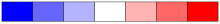
  Bi-polar color progression

• A Spectral progression uses a wide range of hues (possibly the entire color wheel) without intended differences in value. This is most commonly used when there is an order to the values, but it is not a "more vs. less" order, such as seasonality. It is frequently used by non-cartographers in situations where other color progressions would be much more effective.

  

  Full-spectral color progression

• A Qualitative progression uses a scattered set of hues in no particular order, with no intended difference in value. This is most commonly used with nominal categories in a qualitative choropleth map, such as "most prevalent religion."

  

  Qualitative color progression

discrete

• https://mokole.com/palette.html
• https://www.vis4.net/blog/2011/12/avoid-equidistant-hsv-colors/
• https://stackoverflow.com/questions/470690/how-to-automatically-generate-n-distinct-colors

• discrete color gradients
• 
  Grayscale progression
• 
  Single hue progression
• 
  Partial spectral progression
• 
  Bi-polar color progression
• 
  Full-spectral color progression
• 
  Qualitative color progression

2D

• 
• 
• 
• 
• 
• 
• 
• 
• 
• 
• 
• 
• 
• 
• 
• 
• 
• 
• 

gray

Light linear-intensity scale

• a scale with linearly-increasing intensity scale (linear luminance output).
• linearly-increasing encoded luminance signal (linear gamma-compressed luma input)

Linear intensity	I =	0.0	0.1	0.2	0.3	0.4	0.5	0.6	0.7	0.8	0.9	1.0
Linear encoding	VS =	0.0	0.1	0.2	0.3	0.4	0.5	0.6	0.7	0.8	0.9	1.0

gamma

Gamma correction or gamma is a nonlinear operation used to encode and decode luminance or tristimulus values in video or still image systems. Gamma correction is, in the simplest cases, defined by the following power-law expression:

$V_{\text{out}}=AV_{\text{in}}^{\gamma },$

where the non-negative real input value $V_{\text{in}}$ is raised to the power $\gamma$ and multiplied by the constant A to get the output value $V_{\text{out}}$. In the common case of A = 1, inputs and outputs are typically in the range 0–1.

A gamma value

• $\gamma <1$ is sometimes called an encoding gamma, and the process of encoding with this compressive power-law nonlinearity is called gamma compression;
• $\gamma >1$ is called a decoding gamma, and the application of the expansive power-law nonlinearity is called gamma expansion.

The light intensity I is related to the source voltage V_s according to

$I\propto V_{\text{s}}^{\gamma },$

where

• γ is the Greek letter gamma

the inverse transfer function (gamma correction) is

$V_{\text{c}}\propto V_{\text{s}}^{1/\gamma },$

where

• V_c is the corrected voltage
• V_s is the source voltage

For example, from an image sensor that converts photocharge linearly to a voltage. In our CRT example

1/γ is 1/2.2 ≈ 0.45.

A power-law function of 0.43 was experimentally determined by researchers to be the best fit for relating gray light intensity to perceived brightness.

gamma adjustment of sRGB isn't quite just 2.4. They actually have a linear section near black - so it's a piecewise function.

Transfer function ("gamma")

Plot of the sRGB intensities (red), and this function's slope in log-log space (blue), which is the instantaneous gamma. Below a compressed value of 0.04045 or a linear intensity of 0.00313, the curve is linear so the gamma is 1. Behind the red curve is a dashed black curve showing an exact gamma = 2.2 power law.

On an sRGB display, each solid bar should look as bright as the surrounding striped dither. (Note: must be viewed at original, 100% size)

The IEC specification indicates a reference display with a nominal gamma of 2.2, which the sRGB working group determined was representative of the CRTs used with Windows operating systems at the time. The ability to directly display sRGB images on a CRT without any lookup greatly helped sRGB's adoption. Gamma also usefully encodes more data near the black, which reduces visible noise and quantization artifacts.

The standard further defines a optical-electro transfer function (OETF), which defines the conversion of linear light or signal intensity to a gamma-compressed image data. This curve is approximately the inverse of the display's $\gamma ^{2.2}$, but with some adjustments to avoid an infinite slope at zero. Near zero, a $\gamma ^{1/2.4}$ power curve intercepts a straight-line section that leads to zero. This prevents the infinite slope at zero that would occur if a plain power curve was used.

In practice a pure $\gamma ^{2.2}$ may be used with sRGB data with very little difference. This improves computational performance and is referred to as "simple sRGB" by Adobe, This is also most displays transform the encoded image data to the screen.

Computing the transfer function

A straight line that passes through (0,0) is $y={\frac {x}{\Phi }}$, and a gamma curve that passes through (1,1) is $y=\left({\frac {x+A}{1+A}}\right)^{\Gamma }$

If these are joined at the point (X,X/Φ) then:

${\frac {X}{\Phi }}=\left({\frac {X+A}{1+A}}\right)^{\Gamma }$

To avoid a kink where the two segments meet, the derivatives must be equal at this point:

${\frac {1}{\Phi }}=\Gamma \left({\frac {X+A}{1+A}}\right)^{\Gamma -1}\left({\frac {1}{1+A}}\right)$

We now have two equations. If we take the two unknowns to be X and Φ then we can solve to give

$X={\frac {A}{\Gamma -1}},\Phi ={\frac {(1+A)^{\Gamma }(\Gamma -1)^{\Gamma -1}}{(A^{\Gamma -1})(\Gamma ^{\Gamma })}}$

The values A = 0.055 and Γ = 2.4 were chosen so the curve closely resembled the gamma-2.2 curve. This gives X ≈ 0.0392857, Φ ≈ 12.9232102. These values, rounded to X = 0.03928, Φ = 12.92321 sometimes describe sRGB conversion.

Draft publications by sRGB's creators further rounded Φ = 12.92, resulting in a small discontinuity in the curve. Some authors adopted these incorrect values, in part because the draft paper was freely available and the official IEC standard is behind a paywall. For the standard, the rounded value of Φ was kept and X was recomputed as 0.04045 to make the curve continuous, resulting in a slope discontinuity from 1/12.92 below the intersection to 1/12.70 above.

Color calibration

• color calibration in wikipedia
• makeuseof : how-to-calibrate-monitor-colors
• askubuntu question: how-to-calibrate-the-monitor-on-an-ubuntu-system
• help.ubuntu : color-calibrate-screen
• askubuntu question: monitor-calibration-on-20-04
• how-to-calibrate-the-monitor-on-an-ubuntu-system
• x-kom-kalibratory-do-monitorow
• x-kom: jaki-monitor-dla-grafika-komputerowego
• netflix test pattern
• astrosurf: calibrate
• cosmotography : calibrat

dwa rodzaje kalibracji:

• programową (poprzez soft dostarczany przez producenta panelu)
• sprzętową (z pomocą urządzenia pomiarowego, na przykład kalibratora do monitorów).

wynik deltaE po kalibracji

• nie powinien przekraczać 1,5 ( dobrze)
• < 1.0 ( wybornie)

W praktyce lepiej polegać na kalibracji sprzętowej, która zachowuje wszystkie tony, odcienie barw oraz płynną gradację.

Monitory

• z fabryczną kalibracją kolorów ( krzywa gamma jest regulowana w fabryce dla każdej matrycy )
  • Eizo
  • BenQ
• czujnik automatycznej kalibracji, który eliminuje konieczność korzystania z zewnętrznych urządzeń
• rozdzielczości ( 4k )
• gęstość pikseli ( duża to 163 punktów na cal)
• technologia eliminacji migotania obrazu
• tryb ciemni, szczególnie przydatny w postprocessingu
• tryb animacji, dbający o spójność wyświetlanych odcieni
• tryb CAD/CAM uwydatniający najdrobniejsze szczegóły znajdujące się na ekranie monitora
• gamut kolorów : 100% gamutu sRGB

zapisz ustawienia monitora w formie profilu, a najlepiej (jeśli to możliwe) kilku różnych, dopasowanych do konkretnych zastosowań.

Simple monitor tests

Gamma correction test image. Only valid at browser zoom = 100%

This procedure is useful for making a monitor display images approximately correctly, on systems in which profiles are not used (for example, the Firefox browser prior to version 3.0 and many others) or in systems that assume untagged source images are in the sRGB colorspace.

In the test pattern, the intensity of each solid color bar is intended to be the average of the intensities in the surrounding striped dither; therefore, ideally, the solid areas and the dithers should appear equally bright in a system properly adjusted to the indicated gamma.

Normally a graphics card has contrast and brightness control and a transmissive LCD monitor has contrast, brightness, and backlight control. Graphics card and monitor contrast and brightness have an influence on effective gamma, and should not be changed after gamma correction is completed.

The top two bars of the test image help to set correct contrast and brightness values. There are eight three-digit numbers in each bar. A good monitor with proper calibration shows the six numbers on the right in both bars, a cheap monitor shows only four numbers.

Given a desired display-system gamma, if the observer sees the same brightness in the checkered part and in the homogeneous part of every colored area, then the gamma correction is approximately correct. In many cases the gamma correction values for the primary colors are slightly different.

Setting the color temperature or white point is the next step in monitor adjustment.

Before gamma correction the desired gamma and color temperature should be set using the monitor controls. Using the controls for gamma, contrast and brightness, the gamma correction on an LCD can only be done for one specific vertical viewing angle, which implies one specific horizontal line on the monitor, at one specific brightness and contrast level. An ICC profile allows one to adjust the monitor for several brightness levels. The quality (and price) of the monitor determines how much deviation of this operating point still gives a satisfactory gamma correction. Twisted nematic (TN) displays with 6-bit color depth per primary color have lowest quality. In-plane switching (IPS) displays with typically 8-bit color depth are better. Good monitors have 10-bit color depth, have hardware color management and allow hardware calibration with a tristimulus colorimeter. Often a 6bit plus FRC panel is sold as 8bit and a 8bit plus FRC panel is sold as 10bit. FRC is no true replacement for more bits. The 24-bit and 32-bit color depth formats have 8 bits per primary color.

With Microsoft Windows 7 and above the user can set the gamma correction through the display color calibration tool dccw.exe or other programs. These programs create an ICC profile file and load it as default. This makes color management easy. Increase the gamma slider in the dccw program until the last colored area, often the green color, has the same brightness in checkered and homogeneous area. Use the color balance or individual colors gamma correction sliders in the gamma correction programs to adjust the two other colors. Some old graphics card drivers do not load the color Look Up Table correctly after waking up from standby or hibernate mode and show wrong gamma. In this case update the graphics card driver.

On some operating systems running the X Window System, one can set the gamma correction factor (applied to the existing gamma value) by issuing the command xgamma -gamma 0.9 for setting gamma correction factor to 0.9, and xgamma for querying current value of that factor (the default is 1.0). In macOS systems, the gamma and other related screen calibrations are made through the System Preferences.

Scaling and blending

The test image is only valid when displayed "raw", i.e. without scaling (1:1 pixel to screen) and color adjustment, on the screen. It does, however, also serve to point out another widespread problem in software: many programs perform scaling in a color space with gamma, instead of a physically-correct linear space. In a sRGB color space with an approximate gamma of 2.2, the image should show a "2.2" result at 50% size, if the zooming is done linearly. Jonas Berlin has created a "your scaling software sucks/rules" image based on the same principle.

In addition to scaling, the problem also applies to other forms of downsampling (scaling down), such as chroma subsampling in JPEG's gamma-enabled Y′CbCr. WebP solves this problem by calculating the chroma averages in linear space then converting back to a gamma-enabled space; an iterative solution is used for larger images. The same sharp YUV (formerly smart YUV) code is used in sjpeg and optionally in AVIF. Kornelski provides a simpler approximation by luma-based weighted average. Alpha compositing, color gradients, and 3D rendering are also affected by this issue.

Paradoxically, when upsampling (scaling up) an image, the result processed in the "wrong" gamma-enabled space tends to be more aesthetically pleasing. This is because upscaling filters are tuned to minimize the ringing artifacts in a linear space, but human perception is non-linear and better approximated by gamma. An alternative way to trim the artifacts is using a sigmoidal light transfer function, a technique pioneered by GIMP's LoHalo filter and later adopted by madVR.

Calibrate your monitor

Before reviewing the work of authors it is recommended that you calibrate your monitor. If you don't do this, keep in mind that you might not see details in very bright or very dark areas. Also, some monitors may be tinted too much towards a certain color, and not have "neutral" color.

See the image below full screen on a completely black background. You should be able to see at least three of the four circles on this image. If you see four then your brightness setting is on the high side, if you see three, it is fine, but if fewer than three are discernible then it is set too low.

Monitor gamma checkerboard

On a gamma-adjusted display, the four circles in the color image blend into the background when seen from a few feet away. If they do not, you could adjust the gamma setting (found in the computer's settings, not on the display), until they do. This may be very difficult to attain, and a slight error is not detrimental. Uncorrected PC displays usually show the circles darker than the background.

Note that on most consumer LCD displays (laptop or flat screen) viewing angle strongly affects these images - correct adjustment on one part of the screen might be incorrect on another part for a stationary head position. Click on the images for more technical information.

If possible, calibration with a hardware monitor calibrator is recommended.

It is also important to ensure that your browser is displaying images at the correct resolution. To verify this, open the [<tvar name=image>https://upload.wikimedia.org/wikipedia/commons/5/54/Pixel_grid_4000x2000.png</tvar> full 4000x2000 version] of the grid you see at the left. The grid is 8 squares wide by 4 squares high, with the squares measuring 500 pixels on each side. After zooming in to 100%, you should check if it looks reasonable given your monitor resolution. For example, if you have a 1920x1080 monitor, the horizontal width should be just short of covering 4 squares, which would be 2000 pixels. Due to scroll bars, menus, etc. the actual amount of space available will be slightly less than your screen resolution.

Firefox is known for having issues on a Windows computer where the Display setting in Control Panel have been set to anything other than 100% scaling; it is common to have a default of 125% (Medium) for large monitors. This results in Firefox upsampling everything by 25%, causing images to appear less sharp than they really are! To fix this issue, you can either change the scaling factor in Display to 100% or go to about:config (in the URL bar) and change layout.css.devPixelsPerPx to 1.0.

Method for domain coloring

HL plot of z, as per the simple color function example described in the text (left), and the graph of the complex function z³ − 1 (right) using the same color function, showing the three zeros as well as the negative real numbers as pink rays starting at the zeros.

Representing a four dimensional complex mapping with only two variables is undesirable, as methods like projections can result in a loss of information. However, it is possible to add variables that keep the four-dimensional process without requiring a visualization of four dimensions. In this case, the two added variables are visual inputs such as color and brightness because they are naturally two variables easily processed and distinguished by the human eye. This assignment is called a "color function". There are many different color functions used. A common practice is to represent the complex argument (also known as "phase" or "angle") with a hue following the color wheel, and the magnitude by other means, such as brightness or saturation.

Simple color function

The following example colors the origin in black, 1 in green, −1 in magenta, and a point at infinity in white:

${\begin{cases}H&=\arg z+2\pi /3,\\S&=100\%,\\L&=\ell (|z|).\end{cases}}$

There are a number of choices for the function $\ell :[0,\infty )\to [0,1)$. $\ell$ should be strictly monotonic and continuous. Another desirable property is $\ell (1/r)=1-\ell (r)$ such that the inverse of a function is exactly as light as the original function is dark (and the other way around). Possible choices include

• $\ell _{1}(r)={\frac {2}{\pi }}\arctan(r)$ and
• $\ell _{2}(r)={\frac {r^{a}}{r^{a}+1}}$ (with some parameter $a>0$). With $a=2$, this corresponds to the stereographic projection onto the Riemann sphere.

A widespread choice which does not have this property is the function $\ell _{3}(r)=1-a^{|r|}$ (with some parameter $0<a<1$) which for $a=1/2$ and $0\leq r\leq 1$ is very close to $\ell _{1}$.

This approach uses the HSL (hue, saturation, lightness) color model. Saturation is always set at the maximum of 100%. Vivid colors of the rainbow are rotating in a continuous way on the complex unit circle, so the sixth roots of unity (starting with 1) are: green, cyan, blue, magenta, red, and yellow.

Since the HSL color space is not perceptually uniform, one can see streaks of perceived brightness at yellow, cyan, and magenta (even though their absolute values are the same as red, green, and blue) and a halo around L = 1/2. More modern color spaces, e.g, the Lab color space or CIECAM02, correct this, making the images more accurate and less saturated.

Discontinuous color changing

Many color graphs have discontinuities, where instead of evenly changing brightness and color, it suddenly changes, even when the function itself is still smooth. This is done for a variety of reasons such as showing more detail or highlighting certain aspects of a function. This is also sometimes done unintentionally, for example if determining the direction of a complex number first depends on calculating the angle, say in the range [-π, π) and then assigning a color as some function of this angle, then in this case the transition across -π = π could be discontinuous. This kind of artifact rarely contrributes to the usefulness of a graph.

Magnitude growth

A discontinuous color function. In the graph, each discontinuity occurs when $|z|=2^{n}$ for integers n.

Unlike the argument, which has finite range, the magnitude of a complex number can range from 0 to ∞. Therefore, in functions that have large ranges of magnitude, changes in magnitude can sometimes be hard to differentiate when a very large change is also pictured in the graph. This can be remedied with a discontinuous color function which shows a repeating brightness pattern for the magnitude based on a given equation. This allows smaller changes to be easily seen as well as larger changes that "discontinuously jump" to a higher magnitude. In the graph on the right, these discontinuities occur in circles around the center, and show a dimming of the graph that can then start becoming brighter again. A similar color function has been used for the graph on top of the article.

Equations that determine the discontinuities may be linear, such as for every integer magnitude, exponential equations such as every magnitude n where $2^{n}$ is an integer, or any other equation.

Highlighting properties

Discontinuities may be placed where outputs have a certain property to highlight which parts of the graph have that property. For instance, a graph may instead of showing the color cyan jump from green to blue. This causes a discontinuity that is easy to spot, and can highlight lines such as where the argument is zero. Discontinuities may also affect large portions of a graph, such as a graph where the color wheel divides the graph into quadrants. In this way, it is easy to show where each quadrant ends up with relations to others.

Color depth

Color_depth

• 1-bit color = binary image
• 8-bit color = 256 colors, usually from a fully-programmable palette ( VGA)
• 24-bit = True color
• 64-bit color = stores 16-bit R, 16-bit G, 16-bit B and 16-bit A. All integer, no floats

number format

Number type

• integer
• floating point number format
  • Small_Float_Formats in OpenGl and Color formats in OpenGl
  • Half in OpenEXR

store

Image formats to store RGB images with floating point pixels:

• you cannot use PNG ( png64 stores 16-bit R, 16-bit G, 16-bit B and 16-bit A. All integer, no floats), JPEG, TGA or GIF formats
• use either
  • TIFF
  • PFM
  • HDR/EXR formats
  • RGBE image format in wikipedia

processing

For processing such images:

• cannot use these with PIL/Pillow because it doesn't support 32-bit float RGB files.
• use :
  • OpenGl
  • OpenCV
  • scikit-image
  • libvips
  • matplotlib

Dynamic range

Dynamic rang types:

• LDR or SDR
• HDR

Dynamic range of

• image
• display
• print

HDR and:

• tone-mapping

color variations

Variations created by color mixing

• Shades: created by adding black to a base color, increasing its darkness. Shades appear more dramatic and richer
• tints: created by adding white to a base color, increasing its lightness. Tints are likely to look pastel and less intense
• Tones: created by adding gray to a base color, increasing its lightness. Tones looks more sophisticated and complex than base colors

Other:

• Hues: refers to the basic family of a color from red to violet. Hues are variations of a base color on the color wheel
• Temperatures: Color are often divided in cool and warm according to how we perceive them. Greens and blues are cool, whilst reds and yellows are warm

4 categories related to color brightness and saturation:

• vivid (light) = high saturation and brightness
• vivid dark = low brightness
• pastel = low saturation and high brightness
• pale (pastel) dark = low saturation and brightness

Shades

Shades of Color Notice that since (0,0,0) is black and (1,1,1) is white, shades of any particular color are created by moving closer to black or to white. You can use the parametric equation for a linear relationship between two values to make shades of a color darker or lighter.

A parametric equation to calculate a linear change between values A and B:

  C = A + (B-A)*t;  // where t varies between 0 and 1

To change a color (r,g,b) to make it lighter, move it closer to (1,1,1).

  newR = r + (1-r)*t;  // where t varies between 0 and 1
  newG = g + (1-g)*t;  // where t varies between 0 and 1
  newB = b + (1-b)*t;  // where t varies between 0 and 1

To change a color (r,g,b) to make it darker, move it closer to (0,0,0).

  newR = r + (0-r)*t;  // where t varies between 0 and 1
  newG = g + (0-g)*t;  // where t varies between 0 and 1
  newB = b + (0-b)*t;  // where t varies between 0 and 1
  // or
  newR = r*t;  // where t varies between 1 and 0
  newG = g*t;  // where t varies between 1 and 0
  newB = b*t;  // where t varies between 1 and 0

coloring functions

// https://github.com/JPBotelho/Fractal-Megacollection/blob/master/Content/Fractals/Single%20Fractals/FractalOperations.cginc
// Coloring functions (smooth)

float rounddown (in float value)
{
	float roundV = round (value);

	return roundV > value ? round (value - 0.5) : roundV;
}

float LinearColoring (in float2 z, in int iteration, in float power)
{
	return iteration + 1 - log( log ( cabs(z) )   ) / log (rounddown(power));
}

float4 newtonColor (in float smoothIndex, in int channel)
{
	float4 color;

	color[channel] = smoothIndex;

	return color;
}

tints or pastel

Names:

• tints (a mixture of a base color with white )
• pale colors = increased lightness
• pastel colors
• soft or muted type of color
• light color

Effect

• soothing to the eye
• looks less intense, pastel, pale, faded look.
• subtle, modern or sophisticated design

Algorithm

• mix base color with white = heavily tinted with white = desaturated with white
• first generate a random color. Then we sature it a little and mix this color with white color
• in HSV. Take a hue. Desaturate the color a bit( = 80% saturation). Use 100% for value.
• in the HSV color space, have high value and low saturation

# https://mdigi.tools/random-pastel-color/
random_color = { r: Random(0, 255), g: Random(0, 255), b: Random(0, 255) }
pastel_color = random_color.saturate( 10% ).mix( white )

‎

/*
 * https://sighack.com/post/procedural-color-algorithms-color-variations
 * Mix randomly-generated RGB colors with a specified
 * base color. The mixing is performed taking into
 * account a user-specified weight parameter 'w', which
 * specifies what percentage of the final color should
 * come from the base color.
 *
 * A value of 0 for the weight specifies that the 100%
 * of the final RGB components should come from the
 * randomly generated color while a value of 0.5
 * specifies an equal proportion from both the base color
 * and the randomly-generated one.
 */
color rgbMixRandom(color base, float w) {
  float r, g, b;

  /* Check bounds for weight parameter */
  w = w > 1 ? 1 : w;
  w = w < 0 ? 0 : w;

  /* Generate components for a random RGB color */
  r = random(256);
  g = random(256);
  b = random(256);

  /* Mix user-specified color using given weight */
  r = (1-w) * r + w * red(base);
  g = (1-w) * g + w * green(base);
  b = (1-w) * b + w * blue(base);

  return color(r, g, b);
}
‎

color effects

• Category:Optical_phenomena in wikipedia
  • Iridescence

color wheel

• https://theblog.adobe.com/the-power-of-the-palette-why-color-is-key-in-data-visualization-and-how-to-use-it/
• https://opendarkroom.com/color-wheel-rendering/
• https://stackoverflow.com/questions/21490210/how-to-plot-a-colour-wheel-by-using-ggplot
• http://sape.inf.usi.ch/quick-reference/ggplot2/colour
• https://stackoverflow.com/questions/10289279/converting-hsv-circle-code-from-delphi-to-c-sharp
• http://color.support/huecircle.html
• https://weallsew.com/color-wheel-basics/
• http://www.printernational.org/rgb-versus-cmyk.php
• https://github.com/jamesthurley/color-wheel-renderer

Intermediate Colour Values

• color algorithms by Christopher Williams

Smooth colouring requires the ability to obtain a colour in between two colours picked from a discrete palette:

function:   getIntermediateColourValue
parameters: c1(R,G,B), c2(R',G',B'), m: 0 <= m <= 1
return:     [R + m * (R' - R),
             G + m * (G' - G),
             B + m * (B' - B)]

Moebius

Informal description

It is a simple sorting function that places numbers into bins:

• The 0 bin has multiples of square numbers (excluding 1)
• The -1 bin contains every prime number and any number that factors into an odd number of distinct primes
• The 1 bin has any number that factors into an even number of distinct primes

description for programmers

Input

any positive integer n

Output

values in {−1, 0, 1} In particular, \mu(p) = -1μ(p)=−1 for all primes pp.

ellipse

centered at origin and not rotated

NOtation

the equation of a ellipse:

• centered at the origin
• with width = 2a and height = 2b

${\frac {x^{2}}{a^{2}}}+{\frac {y^{2}}{b^{2}}}=1.$

the parametric equation is:

$(x,y)=(a\cos(t),b\sin(t))\quad {\text{for}}\quad 0\leq t\leq 2\pi .$

So explicit equations :

$x(t)=a\cos(t)$

$y(t)=b\sin(t)$

The parameter t :

• is called the eccentric anomaly in astronomy
• is not the angle of $(x(t),y(t))$ with the x-axis
• can be called internal angle of the ellipse

rotated and not moved

Rotation In two dimensions

A counterclockwise rotation of a vector through angle θ. The vector is initially aligned with the x-axis.

In two dimensions, the standard rotation matrix has the following form:

$R(\theta )={\begin{bmatrix}\cos \theta &-\sin \theta \\\sin \theta &\cos \theta \\\end{bmatrix}}$.

This rotates column vectors by means of the following matrix multiplication,

${\begin{bmatrix}x'\\y'\\\end{bmatrix}}={\begin{bmatrix}\cos \theta &-\sin \theta \\\sin \theta &\cos \theta \\\end{bmatrix}}{\begin{bmatrix}x\\y\\\end{bmatrix}}$.

Thus, the new coordinates (x′, y′) of a point (x, y) after rotation are

${\begin{aligned}x'&=x\cos \theta -y\sin \theta \,\\y'&=x\sin \theta +y\cos \theta \,\end{aligned}}$.

result

Center is in the origin ( not shifted or not moved) and rotated:

• center is the origin z = (0, 0)
• $\theta$ is the angle measured from x axis
• The parameter t (called the eccentric anomaly in astronomy) is not the angle of $(x(t),y(t))$ with the x-axis
• a,b are the semi-axis in the x and y directions

$\mathbf {x} =\mathbf {x} (\theta )=x\cos \theta -y\sin \theta$

$\mathbf {y} =\mathbf {y} (\theta )=x\sin \theta +y\cos \theta$

Here

• $\theta$ is fixed ( constant value)
• t is a parameter = independent variable used to parametrise the ellipse

$\mathbf {x} =\mathbf {x} _{\theta }(t)=a\cos \ t\cos \theta -b\sin \ t\sin \theta$

$\mathbf {y} =\mathbf {y} _{\theta }(t)=a\cos \ t\sin \theta +b\sin \ t\cos \theta$

So

${\frac {\mathbf {x} ^{2}}{a^{2}}}+{\frac {\mathbf {y} ^{2}}{b^{2}}}=1.$

${\dfrac {(x\cos \theta -y\sin \theta )^{2}}{a^{2}}}+{\dfrac {(x\sin \theta +y\cos \theta )^{2}}{b^{2}}}=1$

${\dfrac {(a\cos \ t\cos \theta -b\sin \ t\sin \theta )^{2}}{a^{2}}}+{\dfrac {(a\cos \ t\sin \theta +b\sin \ t\cos \theta )^{2}}{b^{2}}}=1$

intersection of 2 ellipses

Intersection = common points

not scaled

2 ellipses:

• both are cetered at origin
• first is not rotated, second is rotated (constant angle theta)
• with the same the aspect ratio r (the ratio of the major axis to the minor axis)

$r={\frac {a}{b}}={\frac {a^{\prime }}{b^{\prime }}}$

${\begin{cases}x=x^{\prime }\\y=y^{\prime }\end{cases}}$

Fix x, then find y:

$x=x\cos \theta -y\sin \theta$

$y={\frac {x\cos \theta -x}{\sin \theta }}$

scaled

Second is scaled by factor s

$s={\frac {a^{\prime }}{a}}={\frac {b^{\prime }}{b}}$

For scaled second ellipse:

• choose point on first ellipse z = ( x,y)
• choose rotation angle theta
• compute s and $t^{\prime }$ of second ellipse such that point

$z^{\prime }=z$

$(x^{\prime },y^{\prime })=(x,y)$

System of 2 equations:

${\begin{cases}x=x^{\prime }\\y=y^{\prime }\end{cases}}$

After substitution for $(x^{\prime },y^{\prime })$

${\begin{cases}x=s\ a\ \cos \ t^{\prime }\cos \theta -s\ b\sin t^{\prime }\sin \theta \\y=s\ a\cos \ t^{\prime }\sin \theta +s\ b\ \sin \ t^{\prime }\cos \theta \end{cases}}$

Solve it for $(s,t^{\prime })$

rotated and moved

Algorithm

• first rotate: apply a general rotation of coordinates transformation to ${\frac {x^{2}}{a^{2}}}+{\frac {y^{2}}{b^{2}}}=1$ to rotate the axes to whatever angle you desire.
• then translate the center to $(h,k)$ by replacing the new x and y by $(x-h)$ and $(y-k)$.

Center not in the origin ( shifted or moved) and rotated:

• center = (cx, cy) = (h,k)
• A is the angle measured from x axis
• cx, cy are the shifts in the x and y directions
• a,b are the semi-axis in the x and y directions

${\frac {x^{2}}{a^{2}}}+{\frac {y^{2}}{b^{2}}}=1.$

${\dfrac {((x-cx)\cos(A)+(y-cy)\sin(A))^{2}}{a^{2}}}+{\dfrac {((x-cx)\sin(A)-(y-cy)\cos(A))^{2}}{b^{2}}}=1$

Horse movies

http://www.horsechannel.com/horse-fun/30-best-horse-movies.aspx

The horse movies

• Sylvester
• Spirit: Stallion of CimarronSpirit
• The Silver Stallion: King of the Wild BrumbiesThe Silver Stallion
• Seabiscuit
• National Velvet
• The Man from Snowy RiverThe Man From Snowy River
• Ladyhawke
• International Velvet
• The Horsemasters
• Hildalgo
• The Electric Horseman
• sA Day at the Races
• Champions
• The Black Stallion Returns
• Black Beauty
• The Story of Seabiscuit
• Something to Talk About
• Shergar
• Phar Lap
• Miracle of the White Stallions
• Let It Ride
• Into the West
• The Horse Whisperer
• The Horse in the Gray Flannel Suit
• Flicka
• Dreamer
• Danny
• Casey's Shadow
• The Black Stallion
• All the Pretty Horses

Sequences

Sequence of complex numbers :

$(z_{k})_{k=0}^{\infty }=(z_{0},z_{1},z_{2},...)$

where :

• $z_{k+1}=f^{4}(z_{k})=f(f(f(f(z_{k}))))=(((z^{2}+c)^{2}+c)^{2}+c)^{2}+c$
• $f(z)=z^{2}+c$
• initial point $z_{0}=-0.0061745136621478+0.4880411715884660*i$
• parameter c $c=0.25+0.5*i$

limit of the sequence is a fixed point $z_{f}$ :

$\lim _{k\to \infty }z_{k}=z_{f}=0.5*i$

but speed up convergence of such sequence is very low :

        k  iteration  distance to fixed  
        0         0  0.0134587590787770
        1         4  0.0134587581012325
       10        40  0.0134587493030271
      100       400  0.0134586612907479
     1000      4000  0.0134577781475032
    10000     40000  0.0134486467159642
   100000    400000  0.0133296117811871
  1000000   4000000  0.0113869977319601 
 10000000  40000000  0.0068052112314813  
100000000 400000000  0.0038334379135754 

I need distance 0.003 to the fixed point.

Is it possible to speed up convergence of such sequence ?

Possible solutions :

• Aitken's delta-squared process
• Shanks transformation
• Richardson extrapolation

ODE

Solutions of ordinary differential equation ( ODE) :

• formal power series

series

• formal power series  : give asymptotic representations of well-defined analytic functions which in our case are “true” solutions of the ODEs.
  • asymptotic series
  • divergent
  • convergent
• trans-series = asymptotic expansion with exponentially small terms

Power series expansion of the Koenigs function

http://mathoverflow.net/questions/157309/power-series-expansion-of-the-koenigs-function

Given a non-zero holomorphic function f fixing 0 which isn't a Mobius transform, the Koenigs function of f, which we'll call h, is the function which linearizes f in the sense that

$h(f(z))=f'(0)h(z)$

I am interested in finding an expression or estimates for $h$ in the case where $f$ is a polynomial of low degree with real coefficients. (I'd be pretty happy with degree 3)

I have heard that there is a way of guessing the power series of $h$. Does anyone know of any references which explain how to do this?

how large is $|f'(0)|$.

There is no simple expression for coefficients or any other simple expression for $h$, even when f is quadratic polynomial $\lambda z+z^{2}$.

However the global behaviour of h when f is a polynomial.

If $|f'(0)|<1$, h is analytic in a neighborhood of 0. It has an analytic continuation to the immediate domain of attraction of $0$, the boundary of this domain is the natural boundary for $h$, and the boundary behaviour of $h$ is relatively well understood.

If $|f'(0)|$ is a root of unity, the equation has no solution, even as a formal series.

If $|f'(0)|=1$ but not a root of unity, a formal power series $h$ exists. Let $f'(0)=e^{2\pi i\alpha}$, then everything depends on the fine Diophantine properties of $\alpha$. For quadratic polynomial $f$, there is a necessary and sufficient condition in terms of $\alpha$ for $h$ to be analytic in a neighborhood of $0$ (Yoccoz got a Fileds medal for this). When analytic, its maximal domain of analyticity is the so-called Siegel disc, and $h$ maps this Siegel disc onto a round disc bijectively.

When $|f'(0)|>1$, $h$ exists but its analytic continuation is not single valued. However the inverse of $h$ has a nice property: it is an entire function of finite order. This result is due to Poincare and Valiron.

For the introduction to the properties of this function see P. Fatou, Sur les equations fonctionnelles, in 3 parts, available on http://www.math.purdue.edu/~eremenko/books-papers.html and G. Valiron, Fonctions analytiques, Paris, Press Universitaires, 1954. For the case $|f'(0)|=1$, see the work of Yoccoz.

It follows from this brief description that there can be no simple expression for $h$ (whatever polynomial $f$ of degree at least $2$ you use). It is easy to obtain a recurrence for coefficients, but it is very complicated, and can hardly be used to study $h$. One exception is the work of Siegel on the case $|f'(0)|=1$. he was able to show that the radius of convergence of the power series is positive for certain $\alpha$ by a kind of direct analysis of this recurrence.

Q

• can we recover the original function, from its asymptotic representation ? See Borel sum

Resurgence theory of Ecalle

" Borel-Ecalle resummation of a transseries exists and is unique, if the Borel transforms of all perturbative series are all “endlessly continuable” = Set of all singularities on all Riemann sheets on Borel plane do not form any natural boundaries. Such transseries are called “resurgent functions”"

"Dynamics of parabolic germs via Resurgence Theory

by Artem Dudko | Stony Brook University Time: 15:00 (Monday, Jan. 21, 2013) Location: BA6183, Bahen Center, 40 St George St Abstract: In this talk I will describe the local dynamics of simple parabolic germs from the point of view of \'Ecalle's Resurgent Theory. By definition, a simple parabolic germ at the origin is a germ of the form F(w)=w+w2+O(w3). The local dynamics of the germ F can be described using Fatou coordinates Φattr,Φrep. These Fatou coordinates share the same asymptotic expansion Φ˜. Moreover, Φattr,Φrep can be obtained from Φ˜ using Borel-Laplace summation. J.~\'Ecalle and S.~Voronin independently constructed a complete set of invariants of analytic conjugacy classes of germs with a parabolic fixed point. I will show how to derive these invariants from Φ˜ using \'Ecalle's Resurgent Theory."

Artem Dudko (University of Toronto) Ecalle-Voronin invariants and Resurgent functions (joint work with David Sauzin) "In my talk I will present Ecalle’s resurgent approach to study of the dynamics of simple parabolic germs near the origin. Consider a simple parabolic germ f (z) = z + z 2 + n≥3 a n z n at the origin. By definition, Fatou coordinates for such germ are the conformal solutions of the equation φ(f (z)) = φ(z)+1 in two regions near the origin, called the attracting and the repelling Fatou petals. This equation has a formal solution φ in terms of divergent series. The series φ gives an asymptotic expansion of the Fatou coordinates. In my talk I will explain the procedure of Borel-Laplace summation which allows to obtain the Fatou coordinates from the series φ. The Borel transform of φ has branched singularities at points 2πik, k ∈ Z. If time allows I will explain a remarkable relation between these singularities and Ecalle-Voronin invariants."

Functions

• resurgent function = Borel-Ecalle resummation of a transseries

Functional equation

Abel functional equation

Give a function $f(z)$ we call the Fatou Coordinate/Abel function $\alpha (z)$ or $\phi (z)$ such that :

$\alpha (f(z))=\alpha (z)+1$

$\phi (f(z))=\phi (z)+1\!$

Solving Abel's functional equation

Fatou coordinate

• "the Fatou coordinate for a parabolic fixed point can be obtained as a limit of some linear function of the solutions to Schroder equation for perturbed mappings with attracting fixed points."
• "the Fatou coordinates can be obtained from $\phi$ using Borel-Laplace summation." with asymptotics $\phi (z)=const+z+A\log z+O(z^{-1})$ at infinity
• the Levy algorithm
• transform Abel’s equation to Schroder’s equation and find the principal solution

"the algorithm used at a parabolic point is different than the Schroeder's equation solution. The equations for the abel function at the parabolic point are well defined, dominated by the (-1/x) term; see the first link in my answer and below. The coefficients are also well defined (not super exponential or anything like that). abel(x+x^2)=-1/x+log(x)-x/2+x^2/3-13x^3/36-+113x^4/240-1187x^5/1800 .....However, the series is divergent, so there is an optimal number of terms to use. But in practice, this is not much of a problem; iterate f^{-1}(x) a few times and convergence vastly improves." – Sheldon L Mar 19 at 18:54

Types

• a Hakim-Fatou coordinate. : "for every petal φ: ∆ → C n of the Fatou flower there exists a injective holomorphic map χ: φ(∆) → C such that χ f (z) = χ(z) + 1 for all z ∈ φ(∆). Definition 2.3: The function χ constructed in the previous theorem is a Hakim-Fatou coordinate." ( Fatou flowers and parabolic curves by Marco Abate )
• Fatou-Lavaurs coordinates
• Fatou-Glutsyuk coordinates
• perturbated/unperturbated coordinate
• formal Fatou coordinate (Jean Ecalle at Orsay) = "Jean Ecalle's formal Abel Series, Fatou Coordinate solution for parabolic points with multiplier=1. This is an asymptotic non-converging series, so there is an optimal number of terms to use, so you may have to iterate f or f−1 a few times to get optimally accurate results, so that the coeffient is closer to the fixed point of zero." Sheldon L

Algorithm for computing

• Abel functional equation
• solution of Abel functional equation is a series $\phi (z)=const+z+Alogz+\sum _{j=1}^{\infty }b_{j}z^{-j}$
• sum of series aproximates Fatou coordinate $\phi (z)$

Examples

z/(1+z)

http://mathoverflow.net/questions/45608/does-the-formal-power-series-solution-to-ffx-sin-x-converge/46765#46765

The correct answer to this belongs to the peculiar world of complex dynamics. See John Milnor, *Dynamics in One Complex Variable*.

First, an example. Begin with $f(z)={\frac {z}{1+z}}$, which has derivative 1 at $z=0$ but, along the positive real axis, is slightly less than $x$ when x > 0.

We want to find a Fatou coordinate, which Milnor (page 107) denotes $\alpha,$ that is infinite at $0$ and otherwise solves what is usually called the Abel functional equation,

$\alpha (f(z))=\alpha (z)+1$

There is only one holomorphic Fatou coordinate up to an additive constant. We take

$\alpha (z)={\frac {1}{z}}$

To get fractional iterates of $f(z)$, with real $0\leq s\leq 1$, we take

$f_{s}(z)=\alpha ^{-1}\left(s+\alpha (z)\right)$

and finally

$f_{s}(z)={\frac {z}{1+sz}}$

The desired semigroup homomorphism holds,

$f_{s}(f_{t}(z))=f_{s+t}(z)$ with $f_0(z) = z$ and $f_1(z) = f(z).$

Alright, the case of $\sin z$ emphasizing the positive real axis is not terribly different, as long as we restrict to the interval $ 0 < x \leq \frac{\pi}{2}.$ For any such $x,$ define $x_0 = x, \; x_1 = \sin x, \; x_2 = \sin \sin x,$ and in general $ x_{n+1} = \sin x_n.$ This sequence approaches 0, and in fact does so for any $z$ in a certain open set around the interval $ 0 < x \leq \frac{\pi}{2}$ that is called a petal.

Now, given a specific $x$ with $x_1 = \sin x$ and $ x_{n+1} = \sin x_n$ it is a result of Jean Ecalle at Orsay that we may take $$ \alpha(x) = \lim_{n \rightarrow \infty} \; \; \; \frac{3}{x_n^2} \; + \; \frac{6 \log x_n}{5} \; + \; \frac{79 x_n^2}{1050} \; + \; \frac{29 x_n^4}{2625} \; - \; n.$$

Note that $\alpha$ actually is defined on $ 0 < x < \pi$ with $\alpha(\pi - x) = \alpha(x),$ but the symmetry also means that the inverse function returns to the interval $ 0 < x \leq \frac{\pi}{2}.$

Before going on, the limit technique in the previous paragraph is given in pages 346-353 of *Iterative Functional Equations* by Marek Kuczma, Bogdan Choczewski, and Roman Ger. The solution is specifically Theorem 8.5.8 of subsection 8.5D, bottom of page 351 to top of page 353. Subsection 8.5A, pages 346-347, about Julia's equation, is part of the development.

As before, we define ( at least for $ 0 < x \leq \frac{\pi}{2}$) the parametrized interpolating functions, $$ f_s (x) = \alpha^{-1} \left( s + \alpha(x) \right) $$

In particular $$ f_{1/2} (x) = \alpha^{-1} \left( \frac{1}{2} + \alpha(x) \right) $$

I calculated all of this last night. First, by the kindness of Daniel Geisler, I have a pdf of the graph of this at:

http://zakuski.math.utsa.edu/~jagy/sine_half.pdf

Note that we use the evident symmetries $ f_{1/2} (-x) = - f_{1/2} (x)$ and $ f_{1/2} (\pi -x) = f_{1/2} (x)$

The result gives an interpolation of functions $f_s(x)$ ending at $ f_1(x)=\sin x$ but beginning at the continuous periodic sawtooth function, $x$ for $ -\frac{\pi}{2} \leq x \leq \frac{\pi}{2},$ then $\pi - x$ for $ \frac{\pi}{2} \leq x \leq \frac{3\pi}{2},$ continue with period $2 \pi.$ We do get $ f_s(f_t(z)) = f_{s + t}(z), $ plus the holomorphicity and symmetry of $\alpha$ show that $f_s(x)$ is analytic on the full open interval $ 0 < x < \pi.$

• • EDIT, TUTORIAL**: Given some $z$ in the complex plane in the interior of the equilateral triangle with vertices at $0, \sqrt 3 + i, \sqrt 3 - i,$ take $z_0 = z, \; \; z_1 = \sin z, \; z_2 = \sin \sin z,$ in general $z_{n+1} = \sin z_n$ and $z_n = \sin^{[n]}(z).$ It does not take long to show that $z_n$ stays within the triangle, and that $z_n \rightarrow 0$ as $n \rightarrow \infty.$

Second, say $\alpha(z)$ is a true Fatou coordinate on the triangle, $\alpha(\sin z) = \alpha(z) + 1,$ although we do not know any specific value. Now, $\alpha(z_1) - 1 = \alpha(\sin z_0) - 1 = \alpha(z_0) + 1 - 1 = \alpha(z_0).$ Also $\alpha(z_2) - 2 = \alpha(\sin(z_1)) - 2 = \alpha(z_1) + 1 - 2 = \alpha(z_1) - 1 = \alpha(z_0).$ Induction, given $\alpha(z_n) - n = \alpha(z_0),$ we have $\alpha(z_{n+1}) - (n+1) = \alpha(\sin z_n) - n - 1 = \alpha(z_n) + 1 - n - 1 = \alpha(z_0).$

So, given $z_n = \sin^{[n]}(z),$ we have $\alpha(z_n) - n = \alpha(z).$

Third , let $L(z) = \frac{3}{z^2}+ \frac{6 \log z}{5} + \frac{79 z^2}{ 1050} + \frac{29 z^4}{2625}$. This is a sort of asymptotic expansion (at 0) for $\alpha(z),$ the error is $| L(z) - \alpha(z) | < c_6 |z|^6.$ It is unlikely that putting more terms on $L(z)$ leads to a convergent series, even in the triangle.

Fourth, given some $ z =z_0$ in the triangle. We know that $z_n \rightarrow 0$. So $| L(z_n) - \alpha(z_n) | < c_6 |z_n|^6.$ Or $| (L(z_n) - n ) - ( \alpha(z_n) - n) | < c_6 |z_n|^6 ,$ finally $$ | (L(z_n) - n ) - \alpha(z) | < c_6 |z_n|^6 .$$ Thus the limit being used is appropriate.

Fifth, there is a bootstrapping effect in use. We have no actual value for $\alpha(z),$ but we can write a formal power series for the solution of a Julia equation for $\lambda(z) = 1 / \alpha'(z),$ that is $\lambda(\sin z ) = \cos z \; \lambda(z).$ The formal power series for $\lambda(z)$ begins (KCG Theorem 8.5.1) with $- z^3 / 6,$ the first term in the power series of $\sin z$ after the initial $z.$ We write several more terms, $$\lambda(z) \asymp - \frac{z^3}{6} - \frac{z^5}{30} - \frac{41 z^7}{3780} - \frac{4 z^9}{945} \cdots.$$ We find the formal reciprocal, $$\frac{1}{\lambda(z)} = \alpha'(z) \asymp -\frac{6}{z^3} + \frac{6}{5 z} + \frac{79 z}{525} + \frac{116 z^3}{2625} + \frac{91543 z^5}{6063750}\cdots.$$ Finally we integrate term by term, $$\alpha(z) \asymp \frac{3}{z^2} + \frac{6 \log z }{5} + \frac{79 z^2}{1050} + \frac{29 z^4}{2625} + \frac{91543 z^6}{36382500}\cdots.$$ and truncate where we like, $$\alpha(z) = \frac{3}{z^2} + \frac{6 \log z }{5} + \frac{79 z^2}{1050} + \frac{29 z^4}{2625} + O(z^6)$$

Numerically, let me give some indication of what happens, in particular to emphasize

$  f_{1/2} (\pi/2) = 1.140179\ldots.$

       x      alpha(x)      f(x)       f(f(x))     sin x       f(f(x))- sin x
   1.570796   2.089608    1.140179    1.000000    1.000000      1.80442e-11
   1.560796   2.089837    1.140095    0.999950    0.999950      1.11629e-09
   1.550796   2.090525    1.139841    0.999800    0.999800      1.42091e-10
   1.540796   2.091672    1.139419    0.999550    0.999550      3.71042e-10
   1.530796   2.093279    1.138828    0.999200    0.999200      1.97844e-10
   1.520796   2.095349    1.138070    0.998750    0.998750      -2.82238e-10
   1.510796   2.097883    1.137144    0.998201    0.998201      -7.31867e-10
   1.500796   2.100884    1.136052    0.997551    0.997551      -1.29813e-09
   1.490796   2.104355    1.134794    0.996802    0.996802      -1.14504e-09
   1.480796   2.108299    1.133372    0.995953    0.995953      9.09416e-11
   1.470796   2.112721    1.131787    0.995004    0.995004      1.57743e-09
   1.460796   2.117625    1.130040    0.993956    0.993956      5.63618e-10
   1.450796   2.123017    1.128133    0.992809    0.992809      -3.00337e-10
   1.440796   2.128902    1.126066    0.991562    0.991562      1.19926e-09
   1.430796   2.135285    1.123843    0.990216    0.990216      2.46512e-09
   1.420796   2.142174    1.121465    0.988771    0.988771      -2.4357e-10
   1.410796   2.149577    1.118932    0.987227    0.987227      -1.01798e-10
   1.400796   2.157500    1.116249    0.985585    0.985585      -1.72108e-10
   1.390796   2.165952    1.113415    0.983844    0.983844      -2.31266e-10
   1.380796   2.174942    1.110434    0.982004    0.982004      -4.08812e-10
   1.370796   2.184481    1.107308    0.980067    0.980067      1.02334e-09
   1.360796   2.194576    1.104038    0.978031    0.978031      3.59356e-10
   1.350796   2.205241    1.100627    0.975897    0.975897      2.36773e-09
   1.340796   2.216486    1.097077    0.973666    0.973666      -1.56162e-10
   1.330796   2.228323    1.093390    0.971338    0.971338      -5.29822e-11
   1.320796   2.240766    1.089569    0.968912    0.968912      8.31102e-10
   1.310796   2.253827    1.085616    0.966390    0.966390      -2.91373e-10
   1.300796   2.267522    1.081532    0.963771    0.963771      -5.45974e-10
   1.290796   2.281865    1.077322    0.961055    0.961055      -1.43066e-10
   1.280796   2.296873    1.072986    0.958244    0.958244      -1.58642e-10
   1.270796   2.312562    1.068526    0.955336    0.955336      -3.14188e-10
   1.260796   2.328950    1.063947    0.952334    0.952334      3.20439e-10
   1.250796   2.346055    1.059248    0.949235    0.949235      4.32107e-10
   1.240796   2.363898    1.054434    0.946042    0.946042      1.49412e-10
   1.230796   2.382498    1.049505    0.942755    0.942755      3.42659e-10
   1.220796   2.401878    1.044464    0.939373    0.939373      4.62813e-10
   1.210796   2.422059    1.039314    0.935897    0.935897      3.63659e-11
   1.200796   2.443066    1.034056    0.932327    0.932327      3.08511e-09
   1.190796   2.464924    1.028693    0.928665    0.928665      -8.44918e-10
   1.180796   2.487659    1.023226    0.924909    0.924909      6.32892e-10
   1.170796   2.511298    1.017658    0.921061    0.921061      -1.80822e-09
   1.160796   2.535871    1.011990    0.917121    0.917121      3.02818e-10
   1.150796   2.561407    1.006225    0.913089    0.913089      -3.52346e-10
   1.140796   2.587938    1.000365    0.908966    0.908966      9.35707e-10
   1.130796   2.615498    0.994410    0.904752    0.904752      -2.54345e-10
   1.120796   2.644121    0.988364    0.900447    0.900447      -6.20484e-10
   1.110796   2.673845    0.982228    0.896052    0.896052      -7.91102e-10
   1.100796   2.704708    0.976004    0.891568    0.891568      -1.62699e-09
   1.090796   2.736749    0.969693    0.886995    0.886995      -5.2244e-10
   1.080796   2.770013    0.963297    0.882333    0.882333      -8.63283e-10
   1.070796   2.804543    0.956818    0.877583    0.877583      -2.85301e-10
   1.060796   2.840386    0.950258    0.872745    0.872745      -1.30496e-10
   1.050796   2.877592    0.943618    0.867819    0.867819      -2.82645e-10
   1.040796   2.916212    0.936899    0.862807    0.862807      8.81083e-10
   1.030796   2.956300    0.930104    0.857709    0.857709      -7.70554e-10
   1.020796   2.997914    0.923233    0.852525    0.852525      1.0091e-09
   1.010796   3.041114    0.916288    0.847255    0.847255      -4.96194e-10
   1.000796   3.085963    0.909270    0.841901    0.841901      6.71018e-10
   0.990796   3.132529    0.902182    0.836463    0.836463      -9.28187e-10
   0.980796   3.180880    0.895023    0.830941    0.830941      -1.45774e-10
   0.970796   3.231092    0.887796    0.825336    0.825336      1.26379e-09
   0.960796   3.283242    0.880502    0.819648    0.819648      -1.84287e-10
   0.950796   3.337412    0.873142    0.813878    0.813878      5.84829e-10
   0.940796   3.393689    0.865718    0.808028    0.808028      -2.81364e-10
   0.930796   3.452165    0.858230    0.802096    0.802096      -1.54149e-10
   0.920796   3.512937    0.850679    0.796084    0.796084      -8.29982e-10
   0.910796   3.576106    0.843068    0.789992    0.789992      3.00744e-10
   0.900796   3.641781    0.835396    0.783822    0.783822      8.10903e-10
   0.890796   3.710076    0.827666    0.777573    0.777573      -1.23505e-10
   0.880796   3.781111    0.819878    0.771246    0.771246      5.31326e-10
   0.870796   3.855015    0.812033    0.764842    0.764842      2.26584e-10
   0.860796   3.931924    0.804132    0.758362    0.758362      3.97021e-10
   0.850796   4.011981    0.796177    0.751806    0.751806      -7.84946e-10
   0.840796   4.095339    0.788168    0.745174    0.745174      -3.03503e-10
   0.830796   4.182159    0.780107    0.738469    0.738469      2.63202e-10
   0.820796   4.272614    0.771994    0.731689    0.731689      -7.36693e-11
   0.810796   4.366886    0.763830    0.724836    0.724836      -1.84604e-10
   0.800796   4.465171    0.755616    0.717911    0.717911      3.22084e-10
   0.790796   4.567674    0.747354    0.710914    0.710914      -2.93204e-10
   0.780796   4.674617    0.739043    0.703845    0.703845      1.58448e-11
   0.770796   4.786234    0.730686    0.696707    0.696707      -8.89497e-10
   0.760796   4.902777    0.722282    0.689498    0.689498      2.40592e-10
   0.750796   5.024513    0.713833    0.682221    0.682221      -3.11017e-10
   0.740796   5.151728    0.705339    0.674876    0.674876      7.32554e-10
   0.730796   5.284728    0.696801    0.667463    0.667463      -1.73919e-10
   0.720796   5.423842    0.688221    0.659983    0.659983      -1.66422e-10
   0.710796   5.569419    0.679599    0.652437    0.652437      5.99509e-10
   0.700796   5.721838    0.670935    0.644827    0.644827      -2.45424e-10
   0.690796   5.881501    0.662231    0.637151    0.637151      -6.29884e-10
   0.680796   6.048843    0.653487    0.629412    0.629412      1.86262e-10
   0.670796   6.224333    0.644704    0.621610    0.621610      -5.04285e-10
   0.660796   6.408471    0.635883    0.613746    0.613746      -6.94697e-12
   0.650796   6.601802    0.627025    0.605820    0.605820      -3.81152e-10
   0.640796   6.804910    0.618129    0.597834    0.597834      4.10222e-10
   0.630796   7.018428    0.609198    0.589788    0.589788      -1.91816e-10
   0.620796   7.243040    0.600231    0.581683    0.581683      -4.90592e-10
   0.610796   7.479486    0.591230    0.573520    0.573520      4.29742e-10
   0.600796   7.728570    0.582195    0.565300    0.565300      -1.38719e-10
   0.590796   7.991165    0.573126    0.557023    0.557023      -4.05081e-10
   0.580796   8.268218    0.564025    0.548690    0.548690      -5.76379e-10
   0.570796   8.560763    0.554892    0.540302    0.540302      1.49155e-10
   0.560796   8.869925    0.545728    0.531861    0.531861      1.0459e-11
   0.550796   9.196935    0.536533    0.523366    0.523366      -1.15537e-10
   0.540796   9.543137    0.527308    0.514819    0.514819      -2.84462e-10
   0.530796   9.910004    0.518054    0.506220    0.506220      6.24335e-11
   0.520796   10.299155    0.508771    0.497571    0.497571      -9.24078e-12
   0.510796   10.712365    0.499460    0.488872    0.488872      8.29491e-11
   0.500796   11.151592    0.490122    0.480124    0.480124      3.31769e-10
   0.490796   11.618996    0.480757    0.471328    0.471328      2.27307e-10
   0.480796   12.116964    0.471366    0.462485    0.462485      3.06434e-10
   0.470796   12.648140    0.461949    0.453596    0.453596      4.77846e-11
   0.460796   13.215459    0.452507    0.444662    0.444662      1.53162e-10
   0.450796   13.822186    0.443041    0.435682    0.435682      -2.87541e-10
   0.440796   14.471963    0.433551    0.426660    0.426660      -5.20332e-11
   0.430796   15.168860    0.424037    0.417595    0.417595      -8.17951e-11
   0.420796   15.917436    0.414501    0.408487    0.408487      -4.6788e-10
   0.410796   16.722816    0.404944    0.399340    0.399340      3.70729e-10
   0.400796   17.590771    0.395364    0.390152    0.390152      -6.97547e-11
   0.390796   18.527825    0.385764    0.380925    0.380925      -2.45522e-10
   0.380796   19.541368    0.376143    0.371660    0.371660      4.09758e-10
   0.370796   20.639804    0.366503    0.362358    0.362358      1.15221e-10
   0.360796   21.832721    0.356843    0.353019    0.353019      -4.75977e-11
   0.350796   23.131092    0.347165    0.343646    0.343646      -4.27696e-10
   0.340796   24.547531    0.337468    0.334238    0.334238      2.12743e-10
   0.330796   26.096586    0.327755    0.324796    0.324796      4.06133e-10
   0.320796   27.795115    0.318024    0.315322    0.315322      -2.71476e-10
   0.310796   29.662732    0.308276    0.305817    0.305817      -3.74988e-10
   0.300796   31.722372    0.298513    0.296281    0.296281      -1.50491e-10
   0.290796   34.000986    0.288734    0.286715    0.286715      2.17798e-11
   0.280796   36.530413    0.278940    0.277121    0.277121      4.538e-10
   0.270796   39.348484    0.269132    0.267499    0.267499      5.24261e-11
   0.260796   42.500432    0.259311    0.257850    0.257850      7.03059e-11
   0.250796   46.040690    0.249475    0.248175    0.248175      -1.83863e-10
   0.240796   50.035239    0.239628    0.238476    0.238476      4.06119e-10
   0.230796   54.564668    0.229768    0.228753    0.228753      -2.56253e-10
   0.220796   59.728239    0.219896    0.219007    0.219007      -7.32657e-11
   0.210796   65.649323    0.210013    0.209239    0.209239      3.43103e-11
   0.200796   72.482783    0.200120    0.199450    0.199450      -1.20351e-10
   0.190796   80.425131    0.190216    0.189641    0.189641      1.07544e-10
   0.180796   89.728726    0.180303    0.179813    0.179813      9.93221e-11
   0.170796   100.721954    0.170380    0.169967    0.169967      2.63903e-10
   0.160796   113.838454    0.160449    0.160104    0.160104      6.74095e-10
   0.150796   129.660347    0.150510    0.150225    0.150225      4.34057e-10
   0.140796   148.983681    0.140563    0.140332    0.140332      -2.90965e-11
   0.130796   172.920186    0.130610    0.130424    0.130424      4.02502e-10
   0.120796   203.060297    0.120649    0.120503    0.120503      -1.85618e-11
   0.110796   241.743576    0.110683    0.110570    0.110570      4.2044e-11
   0.100796   292.525678    0.100711    0.100626    0.100626      -1.73504e-11
   0.090796   361.023855    0.090734    0.090672    0.090672      2.88887e-10
   0.080796   456.537044    0.080752    0.080708    0.080708      -2.90848e-10
   0.070796   595.371955    0.070767    0.070737    0.070737      4.71103e-10
   0.060796   808.285844    0.060778    0.060759    0.060759      -3.90636e-10
   0.050796   1159.094719    0.050785    0.050774    0.050774      3.01403e-11
   0.040796   1798.677124    0.040791    0.040785    0.040785      3.77092e-10
   0.030796   3159.000053    0.030794    0.030791    0.030791      2.4813e-10
   0.020796   6931.973789    0.020796    0.020795    0.020795      2.95307e-10
   0.010796   25732.234731    0.010796    0.010796    0.010796      1.31774e-10
       x       alpha(x)        f(x)        f(f(x))     sin x       f(f(x))- sin x

 [1]: http://oskicat.berkeley.edu/record=b14897585~S1

z^2-3/4

Source

$f_{c}(z)=z^{2}+c$

with

$c=-{\frac {3}{4}}$

Action of second iteration of f map :

$f_{c}^{2}$

near parabolic fixed point is close to translation by 2

in Fatou coordinate near fixed point at infinity .

Affine map $h_{c}$ :

$h_{c}(z)=-i(z+{\frac {1}{2}})$

Computing $h_{c}$ using Maxima CAS :

(%i1) z:zx+zy*%i;
(%o1) %i*zy+zx
(%i2) h:-%i*(z+1/2);
(%o2) −%i*(%i*zy+zx+1/2)
(%i3) realpart(h);
(%o3) zy
(%i4) imagpart(h);
(%o4) −zx−1/2

${\widehat {z}}=h_{c}(z)$

and Fatou coordinate Z :

$Z_{c}({\widehat {z}})=-{\frac {1}{2{\widehat {z}}}}$

Computing Fatou coordinatw with Maxima CAS :

(%i1) z:x+y*%i;
(%o1) %i*y+x
(%i2) a:-1/(2*z^2);
(%o2) −1/(2*(%i*y+x)^2)
(%i3) realpart(a);
(%o3) −x^2−y^2/(2*(y^2+x^2)^2)
(%i4) imagpart(a);
(%o4) (x*y)/(y^2+x^2)^2

and in C function

/*

gcc t.c -Wall



*/


#include <stdio.h>
#include <stdlib.h>
#include <math.h>

double GiveUx(double Zx, double Zy)
{

  double Hx, Hy; 
  double t; // temp 
 // double Ux; // re(fatou coordinate)  
  
  // from z to h 
  Hx= Zy;
  Hy= -Zx - 0.5;
  // from h to u 
  t = Hx*Hx+Hy*Hy;
  return -Hx*Hx - (Hy*Hy)/(2*t*t);
  
}


int main()
{

 double Zcrx= 0.0;
 double ZAx = -0.5;
 double dZ;
 double zx;
 double u;

 int iMax= 20;

int i ; 


dZ = (Zcrx - ZAx)/(iMax);


zx = Zcrx;
for ( i=0; i<iMax+1; ++i)
{  
  zx = Zcrx -  i*dZ;
  u = GiveUx( zx, 0.0);
  printf("i = %d; z = %f; u = %f  \n", i, zx, u); 
   
} 


return 0;
}

the result of not-normalised Fatou coordinate :

i = 0; z = 0.000000; u = -2.000000  
i = 1; z = -0.025000; u = -2.216066  
i = 2; z = -0.050000; u = -2.469136  
i = 3; z = -0.075000; u = -2.768166  
i = 4; z = -0.100000; u = -3.125000  
i = 5; z = -0.125000; u = -3.555556  
i = 6; z = -0.150000; u = -4.081633  
i = 7; z = -0.175000; u = -4.733728  
i = 8; z = -0.200000; u = -5.555556  
i = 9; z = -0.225000; u = -6.611570  
i = 10; z = -0.250000; u = -8.000000  
i = 11; z = -0.275000; u = -9.876543  
i = 12; z = -0.300000; u = -12.500000  
i = 13; z = -0.325000; u = -16.326531  
i = 14; z = -0.350000; u = -22.222222  
i = 15; z = -0.375000; u = -32.000000  
i = 16; z = -0.400000; u = -50.000000  
i = 17; z = -0.425000; u = -88.888889  
i = 18; z = -0.450000; u = -200.000000  
i = 19; z = -0.475000; u = -800.000000  
i = 20; z = -0.500000; u = -nan  

After normalization ( u(zcr) = 0.0 )

/*

gcc t.c -Wall


*/


#include <stdio.h>
#include <stdlib.h>
#include <math.h>

double GiveUx(double Zx, double Zy)
{

  double Hx, Hy; 
  double t; // temp 
 // double Ux; // re(fatou coordinate)  
  
  // from z to h 
  Hx= Zy;
  Hy= -Zx - 0.5;
  // from h to ux 
  t = Hx*Hx+Hy*Hy;
  return -Hx*Hx - (Hy*Hy)/(2*t*t);
  
}


double GiveNormalizedUx(double Zx, double Zy, double ux0)
{
 
return fabs(GiveUx(Zx, Zy)) - fabs(ux0);


}


int main()
{

 // c = ( -0.750000 ; 0.000000 ) 
 double Zcrx= 0.0; // critical point
 double ZAx = -0.5; // alfa fixed point 
 double dZ;
 double zx;
 double u;
 double ux0;

 int iMax= 20;

int i ; 




dZ = (Zcrx - ZAx)/(iMax);
ux0 = GiveUx(Zcrx, 0.0);

zx = Zcrx;
for ( i=0; i<iMax+1; ++i)
{  
  zx = Zcrx -  i*dZ;
  u = GiveNormalizedUx( zx, 0.0, ux0);
  printf("i = %d; z = %f; u = %f  \n", i, zx, u); 
   
} 


return 0;
}

the result :

i = 0; z = 0.000000; u = 0.000000  
i = 1; z = -0.025000; u = 0.216066  
i = 2; z = -0.050000; u = 0.469136  
i = 3; z = -0.075000; u = 0.768166  
i = 4; z = -0.100000; u = 1.125000  
i = 5; z = -0.125000; u = 1.555556  
i = 6; z = -0.150000; u = 2.081633  
i = 7; z = -0.175000; u = 2.733728  
i = 8; z = -0.200000; u = 3.555556  
i = 9; z = -0.225000; u = 4.611570  
i = 10; z = -0.250000; u = 6.000000  
i = 11; z = -0.275000; u = 7.876543  
i = 12; z = -0.300000; u = 10.500000  
i = 13; z = -0.325000; u = 14.326531  
i = 14; z = -0.350000; u = 20.222222  
i = 15; z = -0.375000; u = 30.000000  
i = 16; z = -0.400000; u = 48.000000  
i = 17; z = -0.425000; u = 86.888889  
i = 18; z = -0.450000; u = 198.000000  
i = 19; z = -0.475000; u = 798.000000  
i = 20; z = -0.500000; u = nan

Seems good :

• u(zcr) = 0
• u(fixed point ) = infinity

Inverse function

(%i1) h:-%i*(z+1/2);
(%o1) −%i*(z+1/2)
(%i2) b:-1/(2*h);
(%o2) −%i/(2*(z+1/2))
(%i3) solve(u=b, z);
(%o3) [z=−(u+%i)/(2*u)]
(%i5) s:%o3;
(%o5) [z=−(u+%i)/(2*u)]
(%i6) s:map(rhs,s);
(%o6) [−(u+%i)/(2*u)]
(%i7) realpart(s);
(%o7) [−1/2]
(%i8) imagpart(s);
(%o8) [−1/(2*u)]

Rererences

• Modulus of analytic classification for the generic unfolding of a codimension one resonant diffeomorphism or resonant saddle by C. Rousseau, C. Christopher
• On the existence of attracting domains for maps tangent to the identity by Sara W. Lapan
• http://www.math.purdue.edu/~eremenko/books-papers.html