User:Molybdenumus/statistical ensemble/representations
Representations of statistical ensembles in statistical mechanics[edit]
The precise mathematical expression for a statistical ensemble has a distinct form depending on the type of mechanics under consideration (quantum or classical). In the classical case, the ensemble is a probability distribution over the microstates. In quantum mechanics, this notion, due to von Neumann, is a way of assigning a probability distribution over the results of each complete set of commuting observables. In classical mechanics, the ensemble is instead written as a probability distribution in phase space; the microstates are the result of partitioning phase space into equal-sized units, although the size of these units can be chosen somewhat arbitrarily.
Requirements for representations[edit]
Putting aside for the moment the question of how statistical ensembles are generated operationally, we should be able to perform the following two operations on ensembles A, B of the same system:
- Test whether A, B are statistically equivalent.
- If p is a real number such that 0 < p < 1, then produce a new ensemble by probabilistic sampling from A with probability p and from B with probability 1 – p.
Under certain conditions, therefore, equivalence classes of statistical ensembles have the structure of a convex set.
Quantum mechanical[edit]
A statistical ensemble in quantum mechanics (also known as a mixed state) is most often represented by a density matrix, denoted by . The density matrix provides a fully general tool that can incorporate both quantum uncertainties (present even if the state of the system were completely known) and classical uncertainties (due to a lack of knowledge) in a unified manner. Any physical observable X in quantum mechanics can be written as an operator, X̂. The expectation value of this operator on the statistical ensemble is given by the following trace:
This can be used to evaluate averages (operator X̂), variances (using operator X̂ 2), covariances (using operator X̂Ŷ), etc. The density matrix must always have a trace of 1: (this essentially is the condition that the probabilities must add up to one).
In general, the ensemble evolves over time according to the von Neumann equation.
Equilibrium ensembles (those that do not evolve over time, ) can be written solely as a function of conserved variables. For example, the microcanonical ensemble and canonical ensemble are strictly functions of the total energy, which is measured by the total energy operator Ĥ (Hamiltonian). The grand canonical ensemble is additionally a function of the particle number, measured by the total particle number operator N̂. Such equilibrium ensembles are a diagonal matrix in the orthogonal basis of states that simultaneously diagonalize each conserved variable. In bra–ket notation, the density matrix is
where the |ψi⟩, indexed by i, are the elements of a complete and orthogonal basis. (Note that in other bases, the density matrix is not necessarily diagonal.)
Classical mechanical[edit]

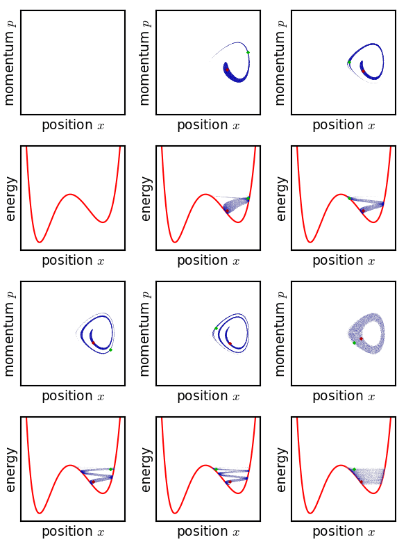
In classical mechanics, an ensemble is represented by a probability density function defined over the system's phase space.[1] While an individual system evolves according to Hamilton's equations, the density function (the ensemble) evolves over time according to Liouville's equation.
In a mechanical system with a defined number of parts, the phase space has n generalized coordinates called q1, ... qn, and n associated canonical momenta called p1, ... pn. The ensemble is then represented by a joint probability density function ρ(p1, ... pn, q1, ... qn).
If the number of parts in the system is allowed to vary among the systems in the ensemble (as in a grand ensemble where the number of particles is a random quantity), then it is a probability distribution over an extended phase space that includes further variables such as particle numbers N1 (first kind of particle), N2 (second kind of particle), and so on up to Ns (the last kind of particle; s is how many different kinds of particles there are). The ensemble is then represented by a joint probability density function ρ(N1, ... Ns, p1, ... pn, q1, ... qn). The number of coordinates n varies with the numbers of particles.
Any mechanical quantity X can be written as a function of the system's phase. The expectation value of any such quantity is given by an integral over the entire phase space of this quantity weighted by ρ:
The condition of probability normalization applies, requiring
Phase space is a continuous space containing an infinite number of distinct physical states within any small region. In order to connect the probability density in phase space to a probability distribution over microstates, it is necessary to somehow partition the phase space into blocks that are distributed representing the different states of the system in a fair way. It turns out that the correct way to do this simply results in equal-sized blocks of canonical phase space, and so a microstate in classical mechanics is an extended region in the phase space of canonical coordinates that has a particular volume.[note 1] In particular, the probability density function in phase space, ρ, is related to the probability distribution over microstates, P by a factor
where
- h is an arbitrary but predetermined constant with the units of energy×time, setting the extent of the microstate and providing correct dimensions to ρ.[note 2]
- C is an overcounting correction factor (see below), generally dependent on the number of particles and similar concerns.
Since h can be chosen arbitrarily, the notional size of a microstate is also arbitrary. Still, the value of h influences the offsets of quantities such as entropy and chemical potential, and so it is important to be consistent with the value of h when comparing different systems.
Cite error: There are <ref group=note> tags on this page, but the references will not show without a {{reflist|group=note}} template (see the help page).


