For help with downloading a single Wikipedia page as a PDF, see Help:Download as PDF.
Advanced Techniques for Biopolymer Structure and Dynamics Contents of Advanced Techniques for Biopolymer Structure and Dynamics
This user book is a user-generated collection of Wikipedia articles that can be easily saved, rendered electronically, and ordered as a printed book. If you are the creator of this book and need help, see Help:Books (general tips) and WikiProject Wikipedia-Books (questions and assistance).
This is an X-ray diffraction pattern formed when X-rays are focused on a crystalline material, in this case a protein. Each dot, called a reflection, forms from the coherent interference of scattered X-rays passing through the crystal.
X-ray scattering techniques are a family of non-destructive analytical techniques which reveal information about the
crystallographic structure, chemical composition, and physical properties of materials and thin films. These techniques are based on observing the
X-ray beam hitting a sample as a function of incident and scattered angle, polarization, and wavelength or energy.
X-ray diffraction techniques
X-ray diffraction finds the geometry or shape of a molecule using X-rays. X-ray
diffraction techniques are based on the elastic scattering of X-rays from structures that have longe range order
crystal. The most comprehensive description of scattering from crystals is given by the
dynamical theory of diffraction.[1]Single-crystal X-ray diffraction is a technique used to solve the complete structure of crystalline materials, ranging from simple inorganic solids to complex
Powder diffraction (XRD) is a technique used to characterize the crystallographic structure, crystallite size (grain size), and preferred orientation in polycrystalline or powdered solid samples. Powder diffraction is commonly used to identify unknown substances, by comparing diffraction data against a database maintained by the
International Centre for Diffraction Data. It may also be used to characterize heterogeneous solid mixtures to determine relative abundance of crystalline compounds and, when coupled with lattice refinement techniques, such as Rietveld refinement, can provide structural information on unknown materials. Powder diffraction is also a common method for determining strains in crystalline materials. An effect of the finite crystallite sizes is seen as a broadening of the peaks in an X-ray diffraction as is explained by the
Thin film diffraction and grazing incidence X-ray diffraction may be used to characterize the crystallographic structure and preferred orientation of substrate-anchored thin films.
High-resolution X-ray diffraction is used to characterize thickness, crystallographic structure, and strain in thin epitaxial films. It employs parallel-beam optics.
X-ray pole figure analysis enables one to analyze and determine the distribution of crystalline orientations within a crystalline thin-film sample.
X-ray rocking curve analysis is used to quantify grain size and mosaic spread in crystalline materials.
Scattering techniques
Elastic scattering
Materials that do not have long range order may also be studied by scattering methods that rely on elastic scattering of monochromatic X-rays.
Small angle X-ray scattering (SAXS) probes structure in the nanometer to micrometer range by measuring scattering intensity at scattering angles 2θ close to 0°.[2]
X-ray reflectivity is an analytical technique for determining thickness, roughness, and density of single layer and multilayer thin films.
When the energy and angle of the inelastically scattered X-rays are monitored scattering techniques can be used to probe the electronic band structure of materials.
Neutron scattering encompasses all scientific techniques whereby the deflection of neutron radiation is used as a scientific probe. Neutrons readily interact with atomic nuclei and magnetic fields from unpaired electrons, making a useful probe of both structure and magnetic order. Neutron Scattering falls into two basic categories - elastic and inelastic. Elastic scattering is when a neutron interacts with a nucleus or electronic magnetic field but does not leave it in an excited state, meaning the emitted neutron has the same energy as the injected neutron. Scattering processes that involve an energetic excitation or relaxation by the neutron are inelastic: the injected neutron's energy is used or increased to create an excitation or by absorbing the excess energy from a relaxation, and consequently the emitted neutron's energy is reduced or increased respectively.
spallation source. Normally in such processes neutrons are however produced with much higher energies than are needed. Therefore moderators are generally used which slow the neutrons down and therefore produce wavelengths that are comparable to the atomic spacing in solids and liquids, and kinetic energies that are comparable to those of dynamic processes in materials. Moderators can be made from Aluminium and filled with liquid hydrogen (for very long wavelength neutrons) or liquid methane (for shorter wavelength neutrons). Fluxes of 107/s - 108/s are not atypical in most neutron sources from any given moderator.
The neutrons cause pronounced interference and energy transfer effects in scattering experiments. Unlike an x-rayphoton with a similar wavelength, which interacts with the electron cloud surrounding the nucleus, neutrons interact with the nucleus itself. Because the neutron is an electrically neutral particle, it is deeply penetrating, and is therefore more able to probe the bulk material. Consequently, it enables the use of a wide range of sample environments that are difficult to use with
synchrotron x-ray sources. It also has the advantage that the cross sections for interaction do not increase with atomic number as they do with radiation from a synchrotron x-ray source. Thus neutrons can be used to analyse materials with low atomic numbers like proteins and surfactants. This can be done at synchrotron sources but very high intensities are needed which may cause the structures to change. Moreover, the nucleus provides a very short range, isotropic potential varying randomly from isotope to isotope, making it possible to tune the nuclear scattering contrast to suit the experiment:
The neutron has an additional advantage over the x-ray photon in the study of condensed matter. It readily interacts with internal magnetic fields in the sample. In fact, the strength of the magnetic scattering signal is often very similar to that of the nuclear scattering signal in many materials, which allows the simultaneous exploration of both nuclear and magnetic structure. Because the neutron scattering amplitude can be measured in absolute units, both the structural and magnetic properties as measured by neutrons can be compared quantitatively with the results of other characterisation techniques.
[[Category:Neutron related techniques]]
[[Category:Scattering]]
[[Category:Neutron]]
Vibrational Circular Dichroism (VCD)
Vibrational circular dichroism (VCD) spectroscopy is basically circular dichroism spectroscopy in the infrared and near infrared ranges[3]. Because VCD is sensitive to the mutual orientation of distinct groups in a molecule, it provides three-dimensional structural information. Thus, it is a powerful technique as VCD spectra of enantiomers can be simulated using ab initio calculations, thereby allowing the identification of absolute configurations of small molecules in solution from VCD spectra. Among such quantum computations of VCD spectra resulting from the chiral properties of small organic molecules are those based on density functional theory (DFT) and gauge-invariant atomic orbitals (GIAO). As a simple example of the experimental results that were obtained by VCD are the spectral data obtained within the carbon-hydrogen (C-H) stretching region of 21 amino acids in heavy water solutions. Measurements of vibrational optical activity (VOA) have thus numerous applications, not only for small molecules, but also for large and complex biopolymers such as muscle proteins (myosin, for example) and DNA.
Vibrational modes
VCD of peptides and proteinsVibrational circular dichroism
Extensive VCD studies have been reported for both polypeptides
and several proteins in solution[4][5][6]; several recent reviews were also compiled[7][8][9][10]. An extensive but not comprehensive VCD publications list is also provided in the "References" section. The published reports over the last 22 years have established VCD as a powerful technique with improved results over those previously obtained by visible/UV circular dichroism (CD) or optical rotatory dispersion (ORD) for proteins and nucleic acids.
Amino acid and polypeptide structures
VCD of nucleic acids
VCD spectra of nucleotides, synthetic polynucleotides and several nucleic acids, including DNA, have been reported and assigned in terms of the type and number of helices present in A- , B-, and Z- DNA.
VCD Instrumentation
For biopolymers such as proteins and nucleic acids, the difference in absorbance between the levo- and dextro- configurations is five orders of magnitude smaller than the
corresonding (unpolarized) absorbance. Therefore, VCD of biopolymers requires the use of very sensitive, specially built instrumentation as well as time-averaging over relatively long intervals of time even with such sensitive VCD spectrometers.
Most CD instruments produce left- and right- circularly polarized light which is then either sine-wave or square-wave modulated, with subsequent phase-sensitive detection and lock-in amplification of the detected signal. In the case of FT-VCD,
a photo-elastic modulator (PEM) is employed in conjunction with an FT-IR interferometer set-up. An example is that of a Bomem model MB-100 FT-IR interferometer equipped with additional polarizing optics/ accessories needed for recording VCD spectra.
A parallel beam emerges through a side port of the interferometer which passes first through a wire grid linear polarizer and then through an octagonal-shaped ZnSe crystal PEM which modulates the polarized beam at a fixed, lower frequency such as 37.5 kHz. A mechanically stressed crystal such as ZnSe exhibits birefringence when stressed by an adjacent piezoelectric transducer. The linear polarizer is positioned close to, and at 45 degrees, with respect to the ZnSe crystal axis. The polarized radiation focused onto the detector is doubly modulated, both by the PEM and by the interferometer setup. A very low noise detector, such as MCT (HgCdTe), is also selected for the VCD signal phase-sensitive detection. Quasi-complete commercial FT-VCD instruments are also available from a few manufacturers but these are quite expensive and also have to be still considered as being at the prototype stage. To prevent detector saturation an appropriate, long wave pass filter is placed before the very low noise MCT detector, which allows only radiation below 1750 cm-1 to reach the MCT detector; the latter however measures radiation only down to 750 cm-1. FT-VCD spectra accumulation of the selected sample solution is then carried out, digitized and stored by an in-line computer. Published reviews that compare various VCD methods are also available.[11][12]
Magnetic VCD
VCD spectra have also been reported in the presence of an applied external magnetic field[13]. This method can enhance the VCD spectral resolution for small molecules[14][15][16][17][18].
Raman optical activity (ROA)
ROA is a technique complementary to VCD especially useful in the 50--1600 cm-1 spectral region; it is considered as the technique of choice for determining optical activity for photon energies less than 600 cm-1.
Notes
^Azároff, L. V. (1974). X-ray diffraction. McGraw-Hill. {{cite book}}: Unknown parameter |coauthors= ignored (|author= suggested) (help)
^*"Vibrational Circular Dichroism of Polypeptides XII. Re-evaluation of the Fourier Transform Vibrational Circular Dichroism of Poly-gamma-Benzyl-L-Glutamate," P. Malon, R. Kobrinskaya, T. A. Keiderling, Biopolymers 27, 733-746 (1988).
^*"Vibrational Circular Dichroism of Biopolymers," T. A. Keiderling, S. C. Yasui, U. Narayanan, A. Annamalai, P. Malon, R. Kobrinskaya, L. Yang, in Spectroscopy of Biological Molecules New Advances ed. E. D. Schmid, F. W. Schneider, F. Siebert, p. 73-76 (1988).
^*"Vibrational Circular Dichroism of Polypeptides and Proteins," S. C. Yasui, T. A. Keiderling, Mikrochimica Acta, II, 325-327, (1988).
^ *"Vibrational Circular Dichroism of Proteins Polysaccharides and Nucleic Acids" T. A. Keiderling, Chapter 8 in Physical Chemistry of Food Processes, Vol. 2 Advanced Techniques, Structures and Applications., eds. I.C. Baianu, H. Pessen, T. Kumosinski, Van Norstrand--Reinhold, New York (1993), pp 307-337.
^ "Spectroscopic characterization of Unfolded peptides and proteins studied with infrared absorption and vibrational circular dichroism spectra" T. A. Keiderling and Qi Xu, Advances in Protein Chemistry Volume 62, [Unfolded Proteins, Dedicated to John Edsall, Ed.: George Rose, Academic Press:New York] (2002), pp. 111-161.
^*"Protein and Peptide Secondary Structure and Conformational Determination with Vibrational Circular Dichroism " Timothy A. Keiderling, Current Opinions in Chemical Biology (Ed. Julie Leary and Mark Arnold) 6, 682-688 (2002).
^*Review: Conformational Studies of Peptides with Infrared Techniques. Timothy A. Keiderling and R. A. G. D. Silva, in Synthesis of Peptides and Peptidomimetics, Ed. M. Goodman and G. Herrman, Houben-Weyl, Vol 22Eb, Georg Thiem Verlag, New York (2002) pp. 715-738, (written and accepted in 2000).
^"Polarization Modulation Fourier Transform Infrared Spectroscopy with Digital SignalProcessing: Comparison of Vibrational Circular Dichroism Methods." Jovencio Hilario, DavidDrapcho, Raul Curbelo, Timothy A. Keiderling, Applied Spectroscopy 55, 1435-1447(2001)--
^ "Vibrational circular dichroism of biopolymers. Summary of methods and applications.", Timothy A. Keiderling, Jan Kubelka, Jovencio Hilario, in Vibrational spectroscopy of polymers and biological systems, Ed. Mark Braiman, Vasilis Gregoriou, Taylor&Francis, Atlanta (CRC Press, Boca Raton, FL) (2006) pp. 253-324 (originally written in 2000, updated in 2003)
^"Observation of Magnetic Vibrational Circular Dichroism," T. A. Keiderling, Journal of Chemical Physics, 75, 3639-41 (1981).
^ "Vibrational Spectral Assignment and Enhanced Resolution Using Magnetic Vibrational Circular Dichroism," T. R. Devine and T. A. Keiderling, Spectrochimica Acta, 43A, 627-629 (1987).
^"Magnetic Vibrational Circular Dichroism with an FTIR" P. V. Croatto, R. K. Yoo, T. A. Keiderling, SPIE Proceedings 1145 (7th International Conference on FTS, ed. D. G. Cameron) 152-153 (1989).
^ "Direct Measurement of the Rotational g-Value in the Ground State of Acetylene by Magnetic Vibrational Circular Dichroism." C. N. Tam and T. A. Keiderling, Chemical Physics Letters, 243, 55-58 (1995).
^. "Ab initio calculation of the vibrational magnetic dipole moment" P. Bour, C. N. Tam, T. A. Keiderling, Journal of Physical Chemistry 99, 17810-17813 (1995)
^ "Rotationally Resolved Magnetic Vibrational Circular Dichroism. Experimental Spectra and Theoretical Simulation for Diamagnetic Molecules." P. Bour, C. N. Tam, B. Wang, T. A. Keiderling, Molecular Physics 87, 299-318, (1996).
ReferencesPeptides and proteins
Huang R, Wu L, McElheny D, Bour P, Roy A, Keiderling TA. Cross-Strand Coupling and Site-Specific Unfolding Thermodynamics of a Trpzip beta-Hairpin Peptide Using (13)C Isotopic Labeling and IR Spectroscopy. The journal of physical chemistry. B. 2009 Apr;113(16):5661-74.
"Vibrational Circular Dichroism of Poly alpha-Benzyl-L-Glutamate," R. D. Singh, and T. A. Keiderling, Biopolymers, 20, 237-40 (1981).
"Vibrational Circular Dichroism of Polypeptides II. Solution Amide II and Deuteration Results," A. C. Sen and T. A. Keiderling, Biopolymers, 23, 1519-32 (1984).
"Vibrational Circular Dichroism of Polypeptides III. Film Studies of Several alpha-Helical and ß-Sheet Polypeptides," A. C. Sen and T. A. Keiderling, Biopolymers, 23, 1533-46 (1984).
"Vibrational Circular Dichroism of Polypeptides IV. Film Studies of L-Alanine Homo Oligopeptides," U. Narayanan, T. A. Keiderling, G. M. Bonora, and C. Toniolo, Biopolymers 24, 1257-63 (1985).
"Vibrational Circular Dichroism of Polypeptides, T. A. Keiderling, S. C. Yasui, A. C. Sen, C. Toniolo, G. M. Bonora, in Peptides Structure and Function, Proceedings of the 9th American Peptide Symposium," ed. C. M. Deber, K. Kopple, V. Hruby; Pie rce Chemical: Rockford, IL; 167-172 (1985).
"Vibrational Circular Dichroism of Polypeptides V. A Study of 310 Helical-Octapeptides" S. C. Yasui, T. A. Keiderling, G. M. Bonora, C. Toniolo, Biopolymers 25, 79-89 (1986).
"Vibrational Circular Dichroism of Polypeptides VI. Polytyrosine alpha-helical and Random Coil Results," S. C. Yasui and T. A. Keiderling, Biopolymers 25, 5-15 (1986).
"Vibrational Circular Dichroism of Polypeptides VII. Film and Solution Studies of alpha-forming Homo-Oligopeptides," U. Narayanan, T. A. Keiderling, G. M. Bonora, C. Toniolo, Journal of the American Chemical Society, 108, 2431-2437 (1986).
"Vibrational Circular Dichroism of Polypeptides VIII. Poly Lysine Conformations as a Function of pH in Aqueous Solution," S. C. Yasui, T. A. Keiderling, Journal of the American Chemical Society, 108, 5576-5581 (1986).
"Vibrational Circular Dichroism of Polypeptides IX. A Study of Chain Length Dependence for 310-Helix Formation in Solution." S. C. Yasui, T. A. Keiderling, F. Formaggio, G. M. Bonora, C. Toniolo, Journal of the American Chemical Society 108, 4988-499 3 (1986).
"Vibrational Circular Dichroism of Biopolymers." T. A. Keiderling, Nature, 322, 851-852 (1986).
"Vibrational Circular Dichroism of Polypeptides X. A Study of alpha-Helical Oligopeptides in Solution." S. C. Yasui, T. A. Keiderling, R. Katachai, Biopolymers 26, 1407-1412 (1987).
"Vibrational Circular Dichroism of Polypeptides XI. Conformation of Poly(L-Lysine(Z)-L-Lysine(Z)-L-1-Pyrenylalanine) and Poly(L-Lysine(Z)-L-Lysine(Z)-L-1-Napthylala-nine) in Solution" S. C. Yasui, T. A. Keiderling, and M. Sisido, Macromolecules 20, 2 403-2406 (1987).
"Vibrational Circular Dichroism of Biopolymers" T. A. Keiderling, S. C. Yasui, A. C. Sen, U. Narayanan, A. Annamalai, P. Malon, R. Kobrinskaya, L. Yang, in "F.E.C.S. Second International Conference on Circular Dichroism, Conference Proceedings," ed. M. Kajtar, L. Eötvös Univ., Budapest, 1987, p. 155-161.
"Vibrational Circular Dichroism of Poly-L-Proline and Other Helical Poly-peptides," R. Kobrinskaya, S. C. Yasui, T. A. Keiderling, in "Peptides: Chemistry and Biology, Proceedings of the 10th American Peptide Symposium," ed. G. R. Marshall, ESCOM, L eiden, 1988, p. 65-67.
"Vibrational Circular Dichroism of Polypeptides with Aromatic Side Chains," S. C. Yasui, T. A. Keiderling, in "Peptides: Chemistry and Biology, Proceedings of the 10th American Peptide Symposium," ed. G. R. Marshall, ESCOM, Leiden, 1988, p. 90-92.
"Vibrational Circular Dichroism of Polypeptides XII. Re-evaluation of the Fourier Transform Vibrational Circular Dichroism of Poly-gamma-Benzyl-L-Glutamate," P. Malon, R. Kobrinskaya, T. A. Keiderling, Biopolymers 27, 733-746 (1988).
"Vibrational Circular Dichroism of Biopolymers," T. A. Keiderling, S. C. Yasui, U. Narayanan, A. Annamalai, P. Malon, R. Kobrinskaya, L. Yang, in Spectroscopy of Biological Molecules New Advances ed. E. D. Schmid, F. W. Schneider, F. Siebert, p. 73-76 (1988).
"Vibrational Circular Dichroism of Polypeptides and Proteins," S. C. Yasui, T. A. Keiderling, Mikrochimica Acta, II, 325-327, (1988).
"(1R,7R)-7-Methyl-6,9,-Diazatricyclo[6,3,0,01,6]Tridecanne-5,10-Dione, A Tricyclic Spirodilactam Containing Non-planar Amide Groups: Synthesis, NMR, Crystal Structure, Absolute Configuration, Electronic and Vibrational Circular Dichroism" P. Malon, C . L. Barness, M. Budesinsky, R. K. Dukor, D. van der Helm, T. A. Keiderling, Z. Koblicova, F. Pavlikova, M. Tichy, K. Blaha, Collections of Czechoslovak Chemical Communications 53, 2447-2472 (1988).
"Vibrational Circular Dichroism of Poly Glutamic Acid" R. K. Dukor, T. A. Keiderling, in Peptides 1988 (ed. G. Jung, E. Bayer) Walter de Gruyter, Berlin (1989) pp 519-521.
"Biopolymer Conformational Studies with Vibrational Circular Dichroism" T. A. Keiderling, S. C. Yasui, P. Pancoska, R. K. Dukor, L. Yang, SPIE Proceeding 1057, ("Biomolecular Spectroscopy," ed. H. H. Mantsch, R. R. Birge) 7-14 (1989).
"Vibrational Circular Dichroism. Comparison of Techniques and Practical Considerations" T. A. Keiderling, in "Practical Fourier Transform Infrared Spectroscopy. Industrial and Laboratory Chemical Analysis," ed. J. R. Ferraro, K. Krishnan (Academic Press, San Diego, 1990) p. 203-284.
"Vibrational Circular Dichroism Study of Unblocked Proline Oligomers," R. K. Dukor, T. A. Keiderling, V. Gut, International Journal of Peptide and Protein Research, 38, 198-203 (1991).
"Reassessment of the Random Coil Conformation. Vibrational CD Study of Proline Oligopeptides and Related Polypeptides" R. K. Dukor and T. A. Keiderling, Biopolymers 31 1747-1761 (1991).
"Vibrational CD of the Amide II band in Some Model Polypeptides and Proteins" V. P. Gupta, T. A. Keiderling, Biopolymers 32 239-248 (1992).
"Vibrational Circular Dichroism of Proteins Polysaccharides and Nucleic Acids" T. A. Keiderling, Chapter 8 in Physical Chemistry of Food Processes, Vol. 2 Advanced Techniques, Structures and Applications., eds. I.C. Baianu, H. Pessen, T. Kumosinski, Van Norstrand--Reinhold, New York (1993), pp 307-337.
"Structural Studies of Biological Macromolecules using Vibrational Circular Dichroism" T. A. Keiderling, P. Pancoska, Chapter 6 in Advances in Spectroscopy Vol. 21, Biomolecular Spectroscopy Part B eds. R. E. Hester, R. J. H. Clarke, John W iley Chichester (1993) pp 267-315.
"Ab Initio Simulations of the Vibrational Circular Dichroism of Coupled Peptides" P. Bour and T. A. Keiderling, Journal of the American Chemical Society 115 9602-9607 (1993).
"Ab initio Simulations of Coupled Peptide Vibrational Circular Dichroism" P. Bour, T. A. Keiderling in "Fifth International Conference on The Spectroscopy of Biological Molecules" Th. Theophanides, J. Anastassopoulou, N. Fotopoulos (Eds), Kluwen Aca demic Publ., Dortrecht, 1993, p. 29-30.
"Vibrational Circular Dichroism Spectroscopy of Peptides and Proteins" T. A. Keiderling, in "Circular Dichroism Interpretations and Applications," K. Nakanishi, N. Berova, R. Woody, Eds., VCH Publishers, New York, (1994) pp 497-521.
"Conformational Study of Sequential Lys-Leu Based Polymers and Oligomers using Vibrational and Electronic Circular Dichroism Spectra" V. Baumruk, D. Huo, R. K. Dukor, T. A. Keiderling, D. LeLeivre and A. Brack Biopolymers 34, 1115-1121 (1994).
"Vibrational Optical Activity of Oligopeptides" T. B. Freedman, L. A. Nafie, T. A. Keiderling Biopolymers (Peptide Science) 37 (ed. C. Toniolo) 265-279 (1995).
"Characterization of ß-bend ribbon spiral forming peptides using electronic and vibrational circular dichroism" G. Yoder, T. A. Keiderling, F. Formaggio, M. Crisma, C. Toniolo Biopolymers 35, 103-111 (1995).
"Vibrational Circular Dichroism as a Tool for Determination of Peptide Secondary Structure" P. Bour, T. A. Keiderling, P. Malon, in "Peptides 1994 (Proceedings of the 23rd European Peptide Symposium,1994," (H.L.S. Maia, ed.), Escom, Le iden 1995, p.517-518.
"Helical Screw Sense of homo-oligopeptides of C-alpha-methylated alpha-amino acids as Determined with Vibrational Circular Dichroism." G. Yoder, T. A. Keiderling, M. Crisma, F. Formaggio, C. Toniolo, J. Kamphuis, Tetrahedron Assymmetry 6, 687 -690 (1995).
"Conformational Study of Linear Alternating and Mixed D- and L-Proline Oligomers Using Electronic and Vibrational CD and Fourier Transform IR." W. Mästle, R. K. Dukor, G. Yoder, T. A. Keiderling Biopolymers 36, 623-631 (1995).
Review: "Vibrational Circular Dichroism Applications to Conformational Analysis of Biomolecules" T. A. Keiderling in Circular Dichroism and the Conformational Analysis of Biomolecules ed. G. D. Fasman, Plenum, New York (1996) p. 555-585.
"Mutarotation studies of Poly L-Proline using FT-IR, Electronic and Vibrational Circular Dichroism" R. K. Dukor, T. A. Keiderling, Biospectroscopy 2, 83-100 (1996).
"Vibrational Circular Dichroism Applications in Proteins and Peptides" T. A. Keiderling, Proceedings of the NATO ASI in Biomolecular Structure and Dynamics, Loutrakii Greece, May 1996, Ed. G. Vergoten (delayed second volume to 1998).
"Transfer of Molecular Property Tensors in Cartesian Coordinates: A new algorithm for simulation of vibrational spectra" Petr Bour, Jana Sopkova, Lucie Bednarova, Petr Malon, T. A. Keiderling, Journal of Computational Chemistry 18, 6 46-659 (1997).
"Vibrational Circular Dichroism Characterization of Alanine-Rich Peptides." Gorm Yoder and Timothy A. Keiderling, "Spectroscopy of Biological Molecules: Modern Trends," Ed. P. Carmona, R. Navarro, A. Hernanz, Kluwer Acad. Pub., Netherlands (1997) p p. 27-28.
"Ionic strength effect on the thermal unfolding of alpha-spectrin peptides." D. Lusitani, N. Menhart, T.A. Keiderling and L. W. M. Fung. Biochemistry 37(1998)16546-16554.
"In search of the earliest events of hCGb folding: structural studies of the 60-87 peptide fragment" S. Sherman, L. Kirnarsky, O. Prakash, H. M. Rogers, R.A.G.D. Silva, T.A. Keiderling, D. Smith, A.M. Hanly, F. Perini, and R.W. Ruddon, American Pep tide Symposium Proceedings, 1997.
"Cold Denaturation Studies of (LKELPKEL)n Peptide Using Vibrational Circular Dichroism and FT-IR". R. A. G. D. Silva, Vladimir Baumruk, Petr Pancoska, T. A. Keiderling, Eric Lacassie, and Yves Trudelle, American Peptide Symposium Proceedings, 1997.
"Simulations of oligopeptide vibrational CD. Effects of isotopic labeling." Petr Bour, Jan Kubelka,T. A. Keiderling Biopolymers 53, 380-395 (2000).
"Site specific conformational determination in thermal unfolding studies of helical peptides using vibrational circular dichroism with isotopic substitution" R. A. G. D. Silva, Jan Kubelka, Petr Bour, Sean M. Decatur, Timothy A. Keiderling, Proceedings of the National Academy of Sciences (PNAS:USA) 97, 8318-8323 (2000).
"Folding studies on the human chorionic gonadotropin b -subunit using optical spectroscopy of peptide fragments" R. A. G. D. Silva, S. A. Sherman, F. Perini, E. Bedows, T. A. Keiderling, Journal of the American Chemical Society, 122, 8623-8630 (2000).
"Peptide and Protein Conformational Studies with Vibrational Circular Dichroism and Related Spectroscopies", Timothy A. Keiderling, (Revised and Expanded Chapter) In Circular Dichroism: Principles and Applications, 2nd Edition. (Eds. K. Nakanishi, N. Berova and R. A. Woody, John Wiley & Sons, New York (2000) p. 621-666.
"Conformation studies with Optical Spectroscopy of peptides taken from hairpin sequences in the Human Chorionic Gonadotropin " R. A. G. D. Silva, S. A. Sherman, E. Bedows, T. A. Keiderling, Peptides for the New Millenium, Proceedings of the 16th American Peptide Symposium, (June, 1999 Minneapolis, MN) Ed.G. B. Fields, J. P. Tam, G. Barany, Kluwer Acad. Pub., Dordrecht,(2000) p. 325-326.
"Analysis of Local Conformation within Helical Peptides via Isotope-Edited Vibrational Spectroscopy." S. M. Decatur, T. A. Keiderling, R. A. G. D.Silva, and P. Bour, Peptides for the New Millenium, Proceedings of the 16th American Peptide Symposium, (June, 1999 Minneapolis, MN) Ed. Ed.G. B. Fields, J. P. Tam, G. Barany, Kluwer Acad. Pub., Dordrecht, (2000) p. 414-416.
"The anomalous infrared amide I intensity distribution in C-13 isotopically labeled peptide beta-sheets comes from extended, multiple stranded structures. An Ab Initio study." Jan Kubelka and T. A. Keiderling , Journal of the American Chemical Society. 123, 6142-6150 (2001).
"Vibrational Circular Dichroism of Peptides and Proteins: Survey of Techniques, Qualitative and Quantitative Analyses, and Applications" Timothy A. Keiderling, Chapter in Infrared and Raman Spectroscopy of Biological Materials, Ed. Bing Yan and H.-U. Gremlich, Marcel Dekker, New York (2001) p.55-100.
"Chirality in peptide vibrations. Ab initio computational studies of length, solvation, hydrogen bond, dipole coupling and isotope effects on vibrational CD. " Jan Kubelka, Petr Bour, R. A. Gangani D. Silva, Sean M. Decatur, Timothy A. Keiderling, ACS Symposium Series 810, ["Chirality: Physical Chemistry," (Ed. Janice Hicks) American Chemical Society, Washington, DC] (2002), pp. 50-64.
"Spectroscopic Characterization of Selected b-Sheet Hairpin Models", J. Hilario, J. Kubelka, F. A. Syud, S. H. Gellman, and T. A. Keiderling. Biopolymers (Biospectroscopy) 67: 233-236 (2002)
" Discrimination between peptide 310- and alpha-helices. Theoretical analysis of the impact of alpha-methyl substitution on experimental spectra " Jan Kubelka, R. A. Gangani D. Silva, and T. A. Keiderling, Journal of the American Chemical Society, 124, 5325-5332 (2002).
"Ab Initio Quantum Mechanical Models of Peptide Helices and their Vibrational Spectra" Petr Bour, Jan Kubelka and T. A. Keiderling, Biopolymers 65, 45-59 (2002).
"Discriminating 310- from alpha-helices. Vibrational and electronic CD and IR Absorption study of related Aib-contining oligopeptides" R. A. Gangani D. Silva, Sritana Yasui, Jan Kubelka, Fernando Formaggio, Marco Crisma, Claudio Toniolo, and Timothy A. Keiderling, Biopolymers 65, 229-243 (2002).
"Spectroscopic characterization of Unfolded peptides and proteins studied with infrared absorption and vibrational circular dichroism spectra" T. A. Keiderling and Qi Xu, Advances in Protein Chemistry Volume 62, [Unfolded Proteins, Dedicated to John Edsall, Ed.: George Rose, Academic Press:New York] (2002), pp. 111-161.
"Protein and Peptide Secondary Structure and Conformational Determination with Vibrational Circular Dichroism " Timothy A. Keiderling, Current Opinions in Chemical Biology (Ed. Julie Leary and Mark Arnold) 6, 682-688 (2002).
Review: Conformational Studies of Peptides with Infrared Techniques. Timothy A. Keiderling and R. A. G. D. Silva, in Synthesis of Peptides and Peptidomimetics, Ed. M. Goodman and G. Herrman, Houben-Weyl, Vol 22Eb, Georg Thiem Verlag, New York (2002) pp. 715-738, (written and accepted in 2000).
"Spectroscopic Studies of Structural Changes in Two beta-Sheet Forming Peptides Show an Ensemble of Structures That Unfold Non-Cooperatively" Serguei V. Kuznetsov, Jovencio Hilario, T. A. Keiderling, Anjum Ansari, Biochemistry, 42 :4321-4332, (2003).
"Optical spectroscopic investigations of model beta-sheet hairpins in aqueous solution" Jovencio Hilario, Jan Kubelka, T. A. Keiderling, Journal of the American Chemical Society 125, 7562-7574 (2003).
"Synthesis and conformational study of homopeptides based on (S)-Bin, a C2-symmetric binapthyl-derived Caa-disubstituted glycine with only axial chirality" J.-P. Mazaleyrat, K. Wright, A. Gaucher, M. Wakselman, S. Oancea, F. Formaggio, C. Toniolo, V. Setnicka, J. Kapitan, T. A. Keiderling, Tetrahedron Asymmetry, 14, 1879-1893 (2003).
"Empirical modeling of the peptide amide I band IR intensity in water solution," Petr Bour, Timothy A. Keiderling, Journal of Chemical Physics, 119, 11253-11262 (2003)
"The Nature of Vibrational Coupling in Helical Peptides: An Isotope Labeling Study” by R. Huang, J. Kubelka, W. Barber-Armstrong, R. A. G. D Silva, S. M. Decatur, and T. A. Keiderling, Journal of the American Chemical Society, 126, 2346-2354 (2004).
"The Complete Chirospectroscopic Signature of the Peptide 310 Helix in Aqueous Solution" Claudio Toniolo, Fernando Formaggio, Sabrina Tognon, Quirinus B. Broxterman, Bernard Kaptein, Rong Huang, Vladimir Setnicka, Timothy A. Keiderling, Iain H. McColl, Lutz Hecht, Laurence D. Barron, Biopolymers 75, 32-45 (2004).
"Induced axial chirality in the biphenyl core for the Ca-tetrasubstituted a-amino acid residue Bip and subsequent propagation of chirality in (Bip)n/Val oligopeptides" J.-P. Mazaleyrat, K. Wright, A. Gaucher, N. Toulemonde, M. Wakselman, S. Oancea, C. Peggion, F. Formaggio, V. Setnicka, T. A. Keiderling, C. Toniolo, Journal of the American Chemical Society 126; 12874-12879 (2004).
Ab initio modeling of amide I coupling in anti-parallel b-sheets and the effect of the 13C isotopic labeling on vibrational spectra” Petr Bour, Timothy A. Keiderling, Journal of Physical Chemistry B, 109, 5348-5357 (2005)
Solvent Effects on IR And VCD Spectra of Helical Peptides: Insights from Ab Initio Spectral Simulations with Explicit Water” Jan Kubelka and Timothy A. Keiderling, Journal of Physical Chemistry B 109, 8231-8243 (2005)
IR Study of Cross-Strand Coupling in a beta-Hairpin Peptide Using Isotopic Labels., Vladimir Setnicka, Rong Huang, Catherine L. Thomas, Marcus A. Etienne, Jan Kubelka, Robert P. Hammer, Timothy A. Keiderling Journal of the American Chemical Society 127, 4992-4993 (2005).
Vibrational spectral simulation for peptides of mixed secondary structure: Method comparisons with the trpzip model hairpin. Petr Bour and Timothy A. Keiderling, Journal of Physical Chemistry B 109, 232687-23697 (2005).
Isotopically labeled peptides provide site-resolved structural data with infrared spectra. Probing the structural limit of optical spectroscopy, Timothy A. Keiderling, Rong Huang, Jan Kubelka, Petr Bour, Vladimir Setnicka, Robert P. Hammer, Marcus *A. Etienne, R. A. Gangani D. Silva, Sean M. Decatur Collections Symposium Series, 8, 42-49 (2005)—["Biologically Active Peptides" IXth Conference, Prague Czech Republic, April 20-22, 2005.
Nucleic acids and polynucleotides
"Application of Vibrational Circular Dichroism to Synthetic Polypeptides and Polynucleic Acids" T. A. Keiderling, S. C. Yasui, R. K. Dukor, L. Yang, Polymer Preprints 30, 423-424 (1989).
"Vibrational Circular Dichroism of Polyribonucleic Acids. A Comparative Study in Aqueous Solution." A. Annamalai and T. A. Keiderling, Journal of the American Chemical Society, 109, 3125-3132 (1987).
"Conformational phase transitions (A-B and B-Z) of DNA and models using vibrational circular dichroism" L. Wang, L. Yang, T. A. Keiderling in Spectroscopy of Biological Molecules., eds. R. E. Hester, R. B. Girling, Special Publication 94 Roya l Society of Chemistry, Cambridge (1991) p. 137-38.
"Vibrational Circular Dichroism of Proteins Polysaccharides and Nucleic Acids" T. A. Keiderling, Chapter 8 in Physical Chemistry of Food Processes, Vol. 2 Advanced Techniques, Structures and Applications eds. I. C. Baianu, H. Pessen, T. Kumosinski, Van Norstrand--Reinhold, New York (1993) pp. 307-337.
"Structural Studies of Biological Macromolecules using Vibrational Circular Dichroism" T. A. Keiderling, P. Pancoska, Chapter 6 in Advances in Spectroscopy Vol. 21, "Biomolecular Spectroscopy Part B" ed. R. E. Hester, R. J. H. Clarke, John W iley Chichester (1993) pp 267-315.
"Detection of Triple Helical Nucleic Acids with Vibrational Circular Dichroism," L. Wang, P. Pancoska, T. A. Keiderling in "Fifth International Conference on The Spectroscopy of Biological Molecules" Th. Theophanides, J. Anastassopoulou, N. Fotopoul os (Eds), Kluwen Academic Publ., Dortrecht, 1993, p. 81-82.
"Helical Nature of Poly (dI-dC) � Poly (dI-dC). Vibrational Circular Dichroism Results" L. Wang and T. A. Keiderling Nucleic Acids Research 21 4127-4132 (1993).
"Detection and Characterization of Triple Helical Pyrimidine-Purine-Pyrimidine Nucleic Acids with Vibrational Circular Dichroism" L. Wang, P. Pancoska, T. A. Keiderling, Biochemistry 33 8428-8435 (1994).
"Vibrational Circular Dichroism of A-, B- and Z- form Nucleic Acids in the PO2- Stretching Region" L. Wang, L. Yang, T. A. Keiderling, Biophysical Journal 67, 2460-2467 (1994).
"Studies of multiple stranded RNA and DNA with FTIR, vibrational and electronic circular dichroism," Zhihua Huang, Lijiang Wang and Timothy A. Keiderling, in Spectrosopy of Biological Molecules, Ed. J. C. Merlin, Kluwer Acad. Pub., Dordrecht, 1995, pp . 321-322.
"Vibrational Circular Dichroism Applications to Conformational Analysis of Biomolecules" T. A. Keiderling in "Circular Dichroism and the Conformational Analysis of Biomolecules" ed G. D. Fasman, Plenum, New York (1996) pp. 555-598.
"Vibrational Circular Dichroism Techniques and Application to Nucleic Acids" T. A. Keiderling, In "Biomolecular Structure and Dynamics", NATO ASI series, Series E: Applied Sciences- Vol.342, Eds: G. Vergoten and T. Theophanides, Kluwer Academ ic Publishers, Dordrecht, The Netherlands,pp. 299-317 (1997).
Paracrystalline materials are defined as having short and medium range ordering in their lattice (similar to the liquid crystal phases) but lacking long-range ordering at least in one direction.[1]
Ordering is the regularity in which atoms appear in a predictable lattice, as measured from one point. In a highly ordered, perfectly crystalline material, or
single crystal, the location of every atom in the structure can be described exactly measuring out from a single origin. Conversely, in a disordered structure such as a liquid or
amorphous solid, the location of the first and perhaps second nearest neighbors can be described from an origin (with some degree of uncertainty) and the ability to predict locations decreases rapidly from there out. The distance at which atom locations can be predicted is referred to as the correlation length . A paracrystalline material exhibits correlation somewhere between the fully amorphous and fully crystalline.
Paracrystalline Model
The paracrystalline model is a revision of the Continuous Random Network model first proposed by W. H. Zachariasen in 1932 [4]. The paracrystal model is defined as highly strained, microcrystalline grains surrounded by fully amorphous material [5]. This is a higher energy state then the continuous random network model. The important distinction between this model and the microcrystalline phases is the lack of defined grain boundaries and highly strained lattice parameters, which makes calculations of molecular and lattice dynamics difficult. A general theory of paracrystals has been formulated in a basic textbook[6] , and then further developed/refined by various authors.
Applications
The paracrystal model has been useful, for example, in describing the state of partially amorphous semiconductor materials after deposition. It has also been successfully applied to: synthetic polymers, liquid crystals, biopoloymers [7],[8] and biomembranes[9].
^Voyles, et al. Structure and physical properties of paracrystalline atomistic models of amorphous silicon. J. Ap. Phys., 90(2001) 4437, doi: 10.1063/1.1407319
^Biswas, P, et al. J. Phys.:Condens. Matter, 19 (2007) 455202, doi:10.1088/0953-8984/19/45/455202
scanning tunneling microscope, was developed by Gerd Binnig and Heinrich Rohrer in the early 1980s, a development that earned them the Nobel Prize for Physics in 1986. Binnig, Quate and Gerber invented the first AFM in 1986. The AFM is one of the foremost tools for imaging, measuring and manipulating matter at the nanoscale. The information is gathered by "feeling" the surface with a mechanical probe. Piezoelectric elements that facilitate tiny but accurate and precise movements on (electronic) command enable the very precise scanning.
Block Diagram of Atomic Force MicroscopeAFM cantilever (after use) in the Scanning Electron Microscope, magnification 1,000 x (image width ~ 100 micrometers)AFM cantilever (after use) in the Scanning Electron Microscope, magnification 3,000 x (image width ~ 30 micrometers)
photothermal microspectroscopy, etc.). Typically, the deflection is measured using a laser spot reflected from the top surface of the cantilever into an array of photodiodes. Other methods that are used include optical interferometry, capacitive sensing or piezoresistive AFM cantilevers. These cantilevers are fabricated with piezoresistive elements that act as a strain gauge. Using a Wheatstone bridge, strain in the AFM cantilever due to deflection can be measured, but this method is not as sensitive as laser deflection or interferometry.
If the tip was scanned at a constant height, a risk would exist that the tip collides with the surface, causing damage. Hence, in most cases a feedback mechanism is employed to adjust the tip-to-sample distance to maintain a constant force between the tip and the sample. Traditionally, the sample is mounted on a piezoelectric tube, that can move the sample in the z direction for maintaining a constant force, and the x and y directions for scanning the sample. Alternatively a 'tripod' configuration of three piezo crystals may be employed, with each responsible for scanning in the x,y and z directions. This eliminates some of the distortion effects seen with a tube scanner. In newer designs, the tip is mounted on a vertical piezo scanner while the sample is being scanned in X and Y using another piezo block. The resulting map of the area s = f(x,y) represents the topography of the sample.
The AFM can be operated in a number of modes, depending on the application. In general, possible imaging modes are divided into static (also called Contact) modes and a variety of dynamic (or non-contact) modes where the cantilever is vibrated.
Imaging modes
The primary modes of operation are static (contact) mode and dynamic mode. In the static mode operation, the static tip deflection is used as a feedback signal. Because the measurement of a static signal is prone to noise and drift, low stiffness cantilevers are used to boost the deflection signal. However, close to the surface of the sample, attractive forces can be quite strong, causing the tip to 'snap-in' to the surface. Thus static mode AFM is almost always done in contact where the overall force is repulsive. Consequently, this technique is typically called 'contact mode'. In contact mode, the force between the tip and the surface is kept constant during scanning by maintaining a constant deflection.
In the dynamic mode, the cantilever is externally oscillated at or close to its fundamental resonancefrequency or a harmonic. The oscillation amplitude, phase and resonance frequency are modified by tip-sample interaction forces; these changes in oscillation with respect to the external reference oscillation provide information about the sample's characteristics.
Schemes for dynamic mode operation include frequency modulation and the more common amplitude modulation. In frequency modulation, changes in the oscillation frequency provide information about tip-sample interactions. Frequency can be measured with very high sensitivity and thus the frequency modulation mode allows for the use of very stiff cantilevers. Stiff cantilevers provide stability very close to the surface and, as a result, this technique was the first AFM technique to provide true atomic resolution in ultra-high vacuum conditions (Giessibl).
In amplitude modulation, changes in the oscillation amplitude or phase provide the feedback signal for imaging. In amplitude modulation, changes in the phase of oscillation can be used to discriminate between different types of materials on the surface. Amplitude modulation can be operated either in the non-contact or in the intermittent contact regime. In ambient conditions, most samples develop a liquid meniscus layer. Because of this, keeping the probe tip close enough to the sample for short-range forces to become detectable while preventing the tip from sticking to the surface presents a major hurdle for the non-contact dynamic mode in ambient conditions. Dynamic contact mode (also called intermittent contact or tapping mode) was developed to bypass this problem (Zhong et al.). In dynamic contact mode, the cantilever is oscillated such that the separation distance between the cantilever tip and the sample surface is modulated.
Amplitude modulation has also been used in the non-contact regime to image with atomic resolution by using very stiff cantilevers and small amplitudes in an ultra-high vacuum environment.
Tapping Mode
Single polymer chains (0.4 nm thick) recorded in a tapping mode under aqueous media with different pH. Green locations of the two-chains-superposition correspond to 0.8 nm thickness (Roiter and Minko, 2005).
In tapping mode the cantilever is driven to oscillate up and down at near its resonance frequency by a small piezoelectric element mounted in the AFM tip holder. The amplitude of this oscillation is greater than 10 nm, typically 100 to 200 nm. Due to the interaction of forces acting on the cantilever when the tip comes close to the surface, Van der Waals force or dipole-dipole interaction, electrostatic forces, etc. cause the amplitude of this oscillation to decrease as the tip gets closer to the sample. An electronic servo uses the piezoelectric actuator to control the height of the cantilever above the sample. The servo adjusts the height to maintain a set cantilever oscillation amplitude as the cantilever is scanned over the sample. A Tapping AFM image is therefore produced by imaging the force of the oscillating contacts of the tip with the sample surface. This is an improvement on conventional contact AFM, in which the cantilever just drags across the surface at constant force and can result in surface damage. Tapping mode is gentle enough even for the visualization of supported lipid bilayers or adsorbed single polymer molecules (for instance, 0.4 nm thick chains of synthetic polyelectrolytes) under liquid medium. At the application of proper scanning parameters, the conformation of single molecules remains unchanged for hours (Roiter and Minko, 2005).
Non-Contact Mode
Here the tip of the cantilever does not contact the sample surface. The cantilever is instead oscillated at a frequency slightly above its resonance frequency where the amplitude of oscillation is typically a few nanometers (<10nm). The van der Waals forces, which are strongest from 1nm to 10nm above the surface, or any other long range force which extends above the surface acts to decrease the resonance frequency of the cantilever. This decrease in resonance frequency combined with the feedback loop system maintains a constant oscillation amplitude or frequency by adjusting the average tip-to-sample distance. Measuring the tip-to-sample distance at each (x,y) data point allows the scanning software to construct a topographic image of the sample surface.
Non-contact mode AFM does not suffer from tip or sample degradation effects that are sometimes observed after taking numerous scans with contact AFM. This makes non-contact AFM preferable to contact AFM for measuring soft samples. In the case of rigid samples, contact and non-contact images may look the same. However, if a few monolayers of adsorbed fluid are lying on the surface of a rigid sample, the images may look quite different. An AFM operating in contact mode will penetrate the liquid layer to image the underlying surface, whereas in non-contact mode an AFM will oscillates above the adsorbed fluid layer to image both the liquid and surface.
AFM -Beam Deflection Detection
Laser light from a solid state diode is reflected off the back of the cantilever and collected by a position sensitive detector (PSD) consisting of two closely spaced photodiodes whose output signal is collected by a differential amplifier.
Angular displacement of cantilever results in one photodiode collecting more light than the other photodiode, producing an output signal (the difference between the photodiode signals normalized by their sum) which is proportional to the deflection of the cantilever. It detects cantilever deflections <1Å (thermal noise limited). A long beam path (several cm) amplifies changes in beam angle.
AFM Beam Deflection Detection
Force spectroscopy
Another major application of AFM (besides imaging) is force spectroscopy, the measurement of force-distance curves. For this method, the AFM tip is extended towards and retracted from the surface as the static deflection of the cantilever is monitored as a function of piezoelectric displacement. These measurements have been used to measure nanoscale contacts, atomic bonding, Van der Waals forces, and Casimir forces, dissolution forces in liquids and single molecule stretching and rupture forces (Hinterdorfer & Dufrêne). Forces of the order of a few pico-Newton can now be routinely measured with a vertical distance resolution of better than 0.1 nanometer.
Problems with the technique include no direct measurement of the tip-sample separation and the common need for low stiffness cantilevers which tend to 'snap' to the surface. The snap-in can be reduced by measuring in liquids or by using stiffer cantilevers, but in the latter case a more sensitive deflection sensor is needed. By applying a small dither to the tip, the stiffness (force gradient) of the bond can be measured as well (Hoffmann et al.).
Identification of individual surface atoms
The AFM can be used to image and manipulate atoms and structures on a variety of surfaces. The atom at the apex of the tip "senses" individual atoms on the underlying surface when it forms incipient chemical bonds with each atom. Because these chemical interactions subtly alter the tip's vibration frequency, they can be detected and mapped.
Physicist Oscar Custance (Osaka University, Graduate School of Engineering, Osaka, Japan) and his team used this principle to distinguish between atoms of silicon, tin and lead on an alloy surface (Nature 2007, 446, 64).
The trick is to first measure these forces precisely for each type of atom expected in the sample. The team found that the tip interacted most strongly with silicon atoms, and interacted 23% and 41% less strongly with tin and lead atoms, respectively. Thus, each different type of atom can be identified in the matrix as the tip is moved across the surface.
Such a technique has been used now in biology and extended recently to cell biology. Forces corresponding to (i) the unbinding of receptor ligand couples (ii) unfolding of proteins (iii) cell adhesion at single cell scale have been gathered.
Advantages and disadvantages
The first Atomic Force Microscope
The AFM has several advantages over the scanning electron microscope (SEM). Unlike the electron microscope which provides a two-dimensional projection or a two-dimensional image of a sample, the AFM provides a true three-dimensional surface profile. Additionally, samples viewed by AFM do not require any special treatments (such as metal/carbon coatings) that would irreversibly change or damage the sample. While an electron microscope needs an expensive vacuum environment for proper operation, most AFM modes can work perfectly well in ambient air or even a liquid environment. This makes it possible to study biological macromolecules and even living organisms. In principle, AFM can provide higher resolution than SEM. It has been shown to give true atomic resolution in ultra-high vacuum (UHV) and, more recently, in liquid environments. High resolution AFM is comparable in resolution to Scanning Tunneling Microscopy and Transmission Electron Microscopy.
A disadvantage of AFM compared with the scanning electron microscope (SEM) is the image size. The SEM can image an area on the order of millimetres by millimetres with a depth of field on the order of millimetres. The AFM can only image a maximum height on the order of micrometres and a maximum scanning area of around 150 by 150 micrometres.
Another inconvenience is that an incorrect choice of tip for the required resolution can lead to image artifacts. Traditionally the AFM could not scan images as fast as an SEM, requiring several minutes for a typical scan, while a SEM is capable of scanning at near real-time (although at relatively low quality) after the chamber is evacuated. The relatively slow rate of scanning during AFM imaging often leads to thermal drift in the image (Lapshin, 2004, 2007), making the AFM microscope less suited for measuring accurate distances between artifacts on the image. However, several fast-acting designs were suggested to increase microscope scanning productivity (Lapshin and Obyedkov, 1993) including what is being termed videoAFM (reasonable quality images are being obtained with videoAFM at video rate - faster than the average SEM). To eliminate image distortions induced by thermodrift, several methods were also proposed (Lapshin, 2004, 2007).
AFM images can also be affected by hysteresis of the piezoelectric material (Lapshin, 1995) and cross-talk between the (x,y,z) axes that may require software enhancement and filtering. Such filtering could "flatten" out real topographical features. However, newer AFM use real-time correction software (for example, feature-oriented scanning, Lapshin, 2004, 2007) or closed-loop scanners which practically eliminate these problems. Some AFM also use separated orthogonal scanners (as opposed to a single tube) which also serve to eliminate cross-talk problems.
Due to the nature of AFM probes, they cannot normally measure steep walls or overhangs. Specially made cantilevers can be modulated sideways as well as up and down (as with dynamic contact and non-contact modes) to measure sidewalls, at the cost of more expensive cantilevers and additional artifacts.
Piezoelectric Scanners
AFM scanners are made from piezoelectric material, which expands and contracts proportionally to an applied voltage. Whether they elongate or contract depends upon the polarity of the voltage applied. The scanner is constructed by combining independently operated piezo electrodes for X, Y, & Z into a single tube, forming a scanner which can manipulate samples and probes with extreme precision in 3 dimensions.
Scanners are characterized by their sensitivity which is the ratio of piezo movement to piezo voltage, i.e. by how much the piezo material extends or contracts per applied volt. Because of differences in material or size, the sensitivity varies from scanner to scanner.
Sensitivity varies non-linearly with respect to scan size. Piezo scanners exhibit more sensitivity at the end than at the beginning of a scan. This causes the forward and reverse scans to behave differently and display hysteresis between the two scan directions. This can be corrected by applying a non-linear voltage to the piezo electrodes to cause linear scanner movement and calibrating the scanner accordingly.
The sensitivity of piezoelectric materials decreases exponentially with time. This causes most of the change in sensitivity to occur in the initial stages of the scanner’s life. Piezoelectric scanners are run for approximately 48 hours before they are shipped from the factory so that they are past the point where we can expect large changes in sensitivity. As the scanner ages, the sensitivity will change less with time and the scanner would seldom require recalibration.
Scanning Probe Microscopy (SPM) is a branch of microscopy that forms images of surfaces using a physical probe that scans the specimen. An image of the surface is obtained by mechanically moving the probe in a raster scan of the specimen, line by line, and recording the probe-surface interaction as a function of position. SPM was founded with the invention of the scanning tunneling microscope in 1981.
Many scanning probe microscopes can image several interactions simultaneously. The manner of using these interactions to obtain an image is generally called a mode.
The resolution varies somewhat from technique to technique, but some probe techniques reach a rather impressive atomic resolution. They owe this largely to the ability of piezoelectric actuators to execute motions with a precision and accuracy at the atomic level or better on electronic command. One could rightly call this family of technique 'piezoelectric techniques'. The other common denominator is that the data are typically obtained as a two-dimensional grid of data points, visualized in false color as a computer image.
Of these techniques AFM and STM are the most commonly used followed by MFM and SNOM/NSOM.
Probe tips
Probe tips are normally made of platinum/iridium or gold. There are two main methods for obtaining a sharp probe tip, acid etching and cutting. The first involves dipping a wire end first into an acid bath and waiting until it has etched through the wire and the lower part drops away. The remained is then removed and the resulting tip is often one atom in diameter. An alternative and much quicker method is to take a thin wire and cut it with a pair of scissors or a scalpel. Testing the tip produced via this method on a sample with a known profile will indicate whether the tip is good or not and a single sharp point is achieved roughly 50% of the time. The problem with this method is that you can end up with a tip that has more than one peak but this will be immediately obvious when you start scanning due to the high level of ghost images.
Advantages of scanning probe microscopy
The resolution of the microscopes is not limited by diffraction, but only by the size of the probe-sample interaction volume (i.e., point spread function), which can be as small as a few picometres. Hence the ability to measure small local differences in object height (like that of 135 picometre steps on <100> silicon) is unparalleled. Laterally the probe-sample interaction extends only across the tip atom or atoms involved in the interaction.
The interaction can be used to modify the sample to create small structures (nanolithography).
Unlike electron microscope methods, specimens do not require a partial vacuum but can be observed in air at standard temperature and pressure or while submerged in a liquid reaction vessel.
Disadvantages of scanning probe microscopy
The detailed shape of the scanning tip is sometimes difficult to determine. Its effect on the resulting data is particularly noticeable if the specimen varies greatly in height over lateral distances of 10 nm or less.
The scanning techniques are generally slower in acquiring images, due to the scanning process. As a result, efforts are being made to greatly improve the scanning rate. Like all scanning techniques, the embedding of spatial information into a time sequence opens the door to uncertainties in metrology, say of lateral spacings and angles, which arise due to time-domain effects like specimen drift, feedback loop oscillation, and mechanical vibration.
The maximum image size is generally smaller.
Scanning probe microscopy is often not useful for examining buried solid-solid or liquid-liquid interfaces.
Chemical imaging is the simultaneous measurement of spectra (chemical information) and images or pictures (spatial information)[1][2] The technique is most often applied to either solid or gel samples, and has applications in chemistry, biology[3][4][5][6][7][8], medicine[9][10], pharmacy[11] (see also for example: Chemical Imaging Without Dyeing), food science, biotechnology[12][13], agriculture and industry (see for example:NIR Chemical Imaging in Pharmaceutical Industry and Pharmaceutical Process Analytical Technology:). NIR, IR and Raman chemical imaging is also referred to as hyperspectral, spectroscopic, spectral or multispectral imaging (also see microspectroscopy). However, other ultra-sensitive and selective, chemical imaging techniques are also in use that involve either UV-visible or fluorescence microspectroscopy. Chemical imaging techniques can be used to analyze samples of all sizes, from the single molecule[14][15] to the cellular level in biology and medicine[16][17][18], and to images of planetary systems in astronomy, but different instrumentation is employed for making observations on such widely different systems.
Chemical imaging instrumentation is composed of three components: a radiation source to illuminate the sample, a spectrally selective element, and usually a detector array (the camera) to collect the images. When many stacked spectral channels (wavelengths) are collected for different locations of the microspectrometer focus on a line or planar array in the focal plane, the data is called hyperspectral; fewer wavelength data sets are called multispectral. The data format is called a hypercube. The data set may be visualized as a three-dimensional block of data spanning two spatial dimensions (x and y), with a series of wavelengths (lambda) making up the third (spectral) axis. The hypercube can be visually and mathematically treated as a series of spectrally resolved images (each image plane corresponding to the image at one wavelength) or a series of spatially resolved spectra. The analyst may choose to view the spectrum measured at a particular spatial location; this is useful for chemical identification. Alternatively, selecting an image plane at a particular wavelength can highlight the spatial distribution of sample components, provided that their spectral signatures are different at the selected wavelength.
Many materials, both manufactured and naturally occurring, derive their functionality from the spatial distribution of sample components. For example, extended release pharmaceutical formulations can be achieved by using a coating that acts as a barrier layer. The release of active ingredient is controlled by the presence of this barrier, and imperfections in the coating, such as discontinuities, may result in altered performance. In the semi-conductor industry, irregularities or contaminants in silicon wafers or printed micro-circuits can lead to failure of these components. The functionality of biological systems is also dependent upon chemical gradients – a single cell, tissue, and even whole organs function because of the very specific arrangement of components. It has been shown that even small changes in chemical composition and distribution may be an early indicator of disease.
Any material that depends on chemical gradients for functionality may be amenable to study by an analytical technique that couples spatial and chemical characterization. To efficiently and effectively design and manufacture such materials, the ‘what’ and the ‘where’ must both be measured. The demand for this type of analysis is increasing as manufactured materials become more complex. Chemical imaging techniques not only permit visualization of the spatially resolved chemical information that is critical to understanding modern manufactured products, but it is also a non-destructive technique so that samples are preserved for further testing.
History
Commercially available laboratory-based chemical imaging systems emerged in the early 1990s (ref. 1-5). In addition to economic factors, such as the need for sophisticated electronics and extremely high-end computers, a significant barrier to commercialization of infrared imaging was that the focal plane array (FPA) needed to read IR images were not readily available as commercial items. As high-speed electronics and sophisticated computers became more commonplace, and infrared cameras became readily commercially available, laboratory chemical imaging systems were introduced.
Initially used for novel research in specialized laboratories, chemical imaging became a more commonplace analytical technique used for general R&D, quality assurance (QA) and quality control (QC) in less than a decade. The rapid acceptance of the technology in a variety of industries (pharmaceutical, polymers, semiconductors, security, forensics and agriculture) rests in the wealth of information characterizing both chemical composition and morphology. The parallel nature of chemical imaging data makes it possible to analyze multiple samples simultaneously for applications that require high throughput analysis in addition to characterizing a single sample.
Principles
Chemical imaging shares the fundamentals of vibrational spectroscopic techniques, but provides additional information by way of the simultaneous acquisition of spatially resolved spectra. It combines the advantages of digital imaging with the attributes of spectroscopic measurements. Briefly, vibrational spectroscopy measures the interaction of light with matter. Photons that interact with a sample are either absorbed or scattered; photons of specific energy are absorbed, and the pattern of absorption provides information, or a fingerprint, on the molecules that are present in the sample.
On the other hand, in terms of the observation setup, chemical imaging can be carried out in one of the following modes: (optical) absorption, emission (fluorescence), (optical) transmission or scattering (Raman). A consensus currently exists that the fluorescence (emission) and Raman scattering modes are the most sensitive and powerful, but also the most expensive.
In a transmission measurement, the radiation goes through a sample and is measured by a detector placed on the far side of the sample. The energy transferred from the incoming radiation to the molecule(s) can be calculated as the difference between the quantity of photons that were emitted by the source and the quantity that is measured by the detector. In a diffuse reflectance measurement, the same energy difference measurement is made, but the source and detector are located on the same side of the sample, and the photons that are measured have re-emerged from the illuminated side of the sample rather than passed through it. The energy may be measured at one or multiple wavelengths; when a series of measurements are made, the response curve is called a spectrum.
A key element in acquiring spectra is that the radiation must somehow be energy selected – either before or after interacting with the sample. Wavelength selection can be accomplished with a fixed filter, tunable filter, spectrograph, an interferometer, or other devices. For a fixed filter approach, it is not efficient to collect a significant number of wavelengths, and multispectral data are usually collected. Interferometer-based chemical imaging requires that entire spectral ranges be collected, and therefore results in hyperspectral data. Tunable filters have the flexibility to provide either multi- or hyperspectral data, depending on analytical requirements.
Spectra may be measured one point at a time using a single element detector (single-point mapping), as a line-image using a linear array detector (typically 16 to 28 pixels) (linear array mapping), or as a two-dimensional image using a Focal Plane Array (FPA)(typically 256 to 16,384 pixels) (FPA imaging). For single-point the sample is moved in the x and y directions point-by-point using a computer-controlled stage. With linear array mapping, the sample is moved line-by-line with a computer-controlled stage. FPA imaging data are collected with a two-dimensional FPA detector, hence capturing the full desired field-of-view at one time for each individual wavelength, without having to move the sample. FPA imaging, with its ability to collected tens of thousands of spectra simultaneously is orders of magnitude faster than linear arrays which are can typically collect 16 to 28 spectra simultaneously, which are in turn much faster than single-point mapping.
Terminology
Some words common in spectroscopy, optical microscopy and photography have been adapted or their scope modified for their use in chemical imaging. They include: resolution, field of view and magnification. There are two types of resolution in chemical imaging. The spectral resolution refers to the ability to resolve small energy differences; it applies to the spectral axis. The spatial resolution is the minimum distance between two objects that is required for them to be detected as distinct objects. The spatial resolution is influenced by the field of view, a physical measure of the size of the area probed by the analysis. In imaging, the field of view is a product of the magnification and the number of pixels in the detector array. The magnification is a ratio of the physical area of the detector array divided by the area of the sample field of view. Higher magnifications for the same detector image a smaller area of the sample.
Types of vibrational chemical imaging instruments
Chemical imaging has been implemented for mid-infrared, near-infrared spectroscopy and
Raman spectroscopy. As with their bulk spectroscopy counterparts, each imaging technique has particular strengths and weaknesses, and are best suited to fulfill different needs.
Mid-infrared chemical imaging
Mid-infrared (MIR) spectroscopy probes fundamental molecular vibrations, which arise in the spectral range 2,500-25,000 nm. Commercial imaging implementations in the MIR region typically employ Fourier Transform Infrared (FT-IR) interferometers and the range is more commonly presented in wavenumber, 4,000 – 400 cm-1. The MIR absorption bands tend to be relatively narrow and well-resolved; direct spectral interpretation is often possible by an experienced spectroscopist. MIR spectroscopy can distinguish subtle changes in chemistry and structure, and is often used for the identification of unknown materials. The absorptions in this spectral range are relatively strong; for this reason, sample presentation is important to limit the amount of material interacting with the incoming radiation in the MIR region. Most data collected in this range is collected in transmission mode through thin sections (~10 micrometres) of material. Water is a very strong absorber of MIR radiation and wet samples often require advanced sampling procedures (such as attenuated total reflectance). Commercial instruments include point and line mapping, and imaging. All employ an FT-IR interferometer as wavelength selective element and light source.
Remote chemical imaging of a simultaneous release of SF6 and NH3 at 1.5km using the FIRST imaging spectrometer[19]For types of MIR microscope, see Microscopy#infrared microscopy.
Atmospheric windows in the infrared spectrum are also employed to perform chemical imaging remotely. In these spectral regions the atmospheric gases (mainly water and CO2) present low absorption and allow infrared viewing over kilometer distances. Target molecules can then be viewed using the selective absorption/emission processes described above. An example of the chemical imaging of a simultaneous release of SF6 and NH3 is shown in the image.
Near-infrared chemical imaging
The analytical near infrared (NIR) region spans the range from approximately 700-2,500 nm. The absorption bands seen in this spectral range arise from overtones and combination bands of O-H, N-H, C-H and S-H stretching and bending vibrations. Absorption is one to two orders of magnitude smaller in the NIR compared to the MIR; this phenomenon eliminates the need for extensive sample preparation. Thick and thin samples can be analyzed without any sample preparation, it is possible to acquire NIR chemical images through some packaging materials, and the technique can be used to examine hydrated samples, within limits. Intact samples can be imaged in transmittance or diffuse reflectance.
The lineshapes for overtone and combination bands tend to be much broader and more overlapped than for the fundamental bands seen in the MIR. Often, multivariate methods are used to separate spectral signatures of sample components. NIR chemical imaging is particularly useful for performing rapid, reproducible and non-destructive analyses of known materials[20][21]. NIR imaging instruments are typically based on one of two platforms: imaging using a tunable filter and broad band illumination, and line mapping employing an FT-IR interferometer as the wavelength filter and light source.
Raman chemical imaging
The Raman shift chemical imaging spectral range spans from approximately 50 to 4,000 cm-1; the actual spectral range over which a particular Raman measurement is made is a function of the laser excitation frequency. The basic principle behind Raman spectroscopy differs from the MIR and NIR in that the x-axis of the Raman spectrum is measured as a function of energy shift (in cm-1) relative to the frequency of the laser used as the source of radiation. Briefly, the Raman spectrum arises from inelastic scattering of incident photons, which requires a change in polarizability with vibration, as opposed to infrared absorption, which requires a change in dipole moment with vibration. The end result is spectral information that is similar and in many cases complementary to the MIR. The Raman effect is weak - only about one in 107 photons incident to the sample undergoes Raman scattering. Both organic and inorganic materials possess a Raman spectrum; they generally produce sharp bands that are chemically specific. Fluorescence is a competing phenomenon and, depending on the sample, can overwhelm the Raman signal, for both bulk spectroscopy and imaging implementations.
Raman chemical imaging requires little or no sample preparation. However, physical sample sectioning may be used to expose the surface of interest, with care taken to obtain a surface that is as flat as possible. The conditions required for a particular measurement dictate the level of invasiveness of the technique, and samples that are sensitive to high power laser radiation may be damaged during analysis. It is relatively insensitive to the presence of water in the sample and is therefore useful for imaging samples that contain water such as biological material.
Fluorescence imaging (visible and NIR)
This emission microspectroscopy mode is the most sensitive
in both visible and FT-NIR microspectroscopy, and has therefore numerous biomedical, biotechnological and agricultural applications. There are several powerful, highly specific and sensitive fluorescence techniques that are currently in use, or still being developed; among the former are FLIM, FRAP, FRET and FLIM-FRET; among the latter are
NIR fluorescence and probe-sensitivity enhanced NIR fluorescence microspectroscopy and nanospectroscopy techniques (see "Further reading" section).
Sampling and samples
The value of imaging lies in the ability to resolve spatial heterogeneities in solid-state or gel/gel-like samples. Imaging a liquid or even a suspension has limited use as constant sample motion serves to average spatial information, unless ultra-fast recording techniques are employed as in fluorescence correlation microspectroscopy or FLIM obsevations where a single molecule may be monitored at extremely high (photon) detection speed. High-throughput experiments (such as imaging multi-well plates) of liquid samples can however provide valuable information. In this case, the parallel acquisition of thousands of spectra can be used to compare differences between samples, rather than the more common implementation of exploring spatial heterogeneity within a single sample.
Similarly, there is no benefit in imaging a truly homogeneous sample, as a single point spectrometer will generate the same spectral information. Of course the definition of homogeneity is dependent on the spatial resolution of the imaging system employed. For MIR imaging, where wavelengths span from 3-10 micrometres, objects on the order of 5 micrometres may theoretically be resolved. The sampled areas are limited by current experimental implementations because illumination is provided by the interferometer. Raman imaging may be able to resolve particles less than 1 micrometre in size, but the sample area that can be illuminated is severely limited. With Raman imaging, it is considered impractical to image large areas and, consequently, large samples. FT-NIR chemical/hyperspectral imaging usually resolves only larger objects (>10 micrometres), and is better suited for large samples because illumination sources are readily available. However, FT-NIR microspectroscopy was recently reported to be capable of about 1.2 micron (micrometer) resolution in biological samples[22] Furthermore, two-photon excitation FCS experiments were reported to have attained 15 nanometer resolution on biomembrane thin films with a special coincidence photon-counting setup.
Detection limits
The concept of the detection limit for chemical imaging is quite different than for bulk spectroscopy, as it depends on the sample itself. Because a bulk spectrum represents an average of the materials present, the spectral signatures of trace components are simply overwhelmed by dilution. In imaging however, each pixel has a corresponding spectrum. If the physical size of the trace contaminant is on the order of the pixel size imaged on the sample, its spectral signature will likely be detectable. If however, the trace component is dispersed homogeneously (relative to pixel image size) throughout a sample, it will not be detectable. Therefore, detection limits of chemical imaging techniques are strongly influenced by particle size, the chemical and spatial heterogeneity of the sample, and the spatial resolution of the image.
Data analysis
Data analysis methods for chemical imaging data sets typically employ mathematical algorithms common to single point spectroscopy or to image analysis. The reasoning is that the spectrum acquired by each detector is equivalent to a single point spectrum; therefore pre-processing, chemometrics and pattern recognition techniques are utilized with the similar goal to separate chemical and physical effects and perform a qualitative or quantitative characterization of individual sample components. In the spatial dimension, each chemical image is equivalent to a digital image and standard image analysis and robust statistical analysis can be used for feature extraction.
^C.L. Evans and X.S. Xie.2008. Coherent Anti-Stokes Raman Scattering Microscopy: Chemical Imaging for Biology and Medicine.,
doi:10.1146/annurev.anchem.1.031207.112754 Annual Review of Analytical Chemistry, 1: 883-909.
^Diaspro, A., and Robello, M. (1999). Multi-photon Excitation Microscopy to Study Biosystems. European Microscopy and Analysis., 5:5-7.
^D.S. Mantus and G. H. Morrison. 1991. Chemical imaging in biology and medicine using ion microscopy., Microchimica Acta, 104, (1-6) January 1991, doi: 10.1007/BF01245536
^Bagatolli, L.A., and Gratton, E. (2000). Two-photon fluorescence microscopy of coexisting lipid domains in giant unilamellar vesicles of binary phospholipid mixtures. Biophys J., 78:290-305.
^Schwille, P., Haupts, U., Maiti, S., and Webb. W.(1999). Molecular dynamics in living cells observed by fluorescence correlation spectroscopy with one- and two-photon excitation. Biophysical Journal, 77(10):2251-2265.
^1.Lee, S. C. et al., (2001). One Micrometer Resolution NMR Microscopy. J. Magn. Res., 150: 207-213.
^Near Infrared Microspectroscopy, Fluorescence Microspectroscopy,Infrared Chemical Imaging and High Resolution Nuclear Magnetic Resonance Analysis of Soybean Seeds, Somatic Embryos and Single Cells., Baianu, I.C. et al. 2004., In Oil Extraction and Analysis., D. Luthria, Editor pp.241-273, AOCS Press., Champaign, IL.
^Single Cancer Cell Detection by Near Infrared Microspectroscopy, Infrared Chemical Imaging and Fluorescence Microspectroscopy.2004.I. C. Baianu, D. Costescu, N. E. Hofmann and S. S. Korban, q-bio/0407006 (July 2004)
^J. Dubois, G. Sando, E. N. Lewis, Near-Infrared Chemical Imaging, A Valuable Tool for the Pharmaceutical Industry, G.I.T. Laboratory Journal Europe, No. 1-2, 2007.
^Raghavachari, R., Editor. 2001. Near-Infrared Applications in Biotechnology, Marcel-Dekker, New York, NY.
^Applications of Novel Techniques to Health Foods, Medical and Agricultural Biotechnology.(June 2004)
I. C. Baianu, P. R. Lozano, V. I. Prisecaru and H. C. Lin
q-bio/0406047
^Eigen, M., and Rigler, R. (1994). Sorting single molecules: Applications to diagnostics and evolutionary biotechnology, Proc. Natl. Acad. Sci. USA 91:5740.
^Rigler R. and Widengren J. (1990). Ultrasensitive detection of single molecules by fluorescence correlation spectroscopy, BioScience (Ed. Klinge & Owman) p.180.
^Single Cancer Cell Detection by Near Infrared Microspectroscopy, Infrared Chemical Imaging and Fluorescence Microspectroscopy.2004.I. C. Baianu, D. Costescu, N. E. Hofmann, S. S. Korban and et al., q-bio/0407006 (July 2004)
^Oehlenschläger F., Schwille P. and Eigen M. (1996). Detection of HIV-1 RNA by nucleic acid sequence-based amplification combined with fluorescence correlation spectroscopy, Proc. Natl. Acad. Sci. USA93:1281.
^Near Infrared Microspectroscopy, Fluorescence Microspectroscopy,Infrared Chemical Imaging and High Resolution Nuclear Magnetic Resonance Analysis of Soybean Seeds, Somatic Embryos and Single Cells., Baianu, I.C. et al. 2004., In Oil Extraction and Analysis., D. Luthria, Editor pp.241-273, AOCS Press., Champaign, IL.
^M. Chamberland, V. Farley, A. Vallières, L. Belhumeur, A. Villemaire, J. Giroux et J. Legault, High-Performance Field-Portable Imaging Radiometric Spectrometer Technology For Hyperspectral imaging Applications, Proc. SPIE 5994, 59940N, September 2005.
^Novel Techniques for Microspectroscopy and Chemical Imaging Analysis of Soybean Seeds and Embryos.(2002). Baianu, I.C., Costescu, D.M., and You, T. Soy2002 Conference, Urbana, Illinois.
^Near Infrared Microspectroscopy, Chemical Imaging and NMR Analysis of Oil in Developing and Mutagenized Soybean Embryos in Culture. (2003). Baianu, I.C., Costescu, D.M., Hofmann, N., and Korban, S.S. AOCS Meeting, Analytical Division.
^Near Infrared Microspectroscopy, Fluorescence Microspectroscopy,Infrared Chemical Imaging and High Resolution Nuclear Magnetic Resonance Analysis of Soybean Seeds, Somatic Embryos and Single Cells., Baianu, I.C. et al. 2004., In Oil Extraction and Analysis., D. Luthria, Editor pp.241-273, AOCS Press., Champaign, IL.
Further reading
E. N. Lewis, P. J. Treado, I. W. Levin, Near-Infrared and Raman Spectroscopic Imaging, American Laboratory, 06/1994:16 (1994)
E. N. Lewis, P. J. Treado, R. C. Reeder, G. M. Story, A. E. Dowrey, C. Marcott, I. W. Levin, FTIR spectroscopic imaging using an infrared focal-plane array detector, Analytical Chemistry, 67:3377 (1995)
P. Colarusso, L. H. Kidder, I. W. Levin, J. C. Fraser, E. N. Lewis Infrared Spectroscopic Imaging: from Planetary to Cellular Systems, Applied Spectroscopy, 52 (3):106A (1998)
P. J. Treado I. W. Levin, E. N. Lewis, Near-Infrared Spectroscopic Imaging Microscopy of Biological Materials Using an Infrared Focal-Plane Array and an Acousto-Optic Tunable Filter (AOTF), Applied Spectroscopy, 48:5 (1994)
Hammond, S.V., Clarke, F. C., Near-infrared microspectroscopy. In: Handbook of Vibrational Spectroscopy, Vol. 2, J.M. Chalmers and P.R. Griffiths Eds. John Wiley and Sons, West Sussex, UK, 2002, p.1405-1418
L.H. Kidder, A.S. Haka, E.N. Lewis, Instrumentation for FT-IR Imaging. In: Handbook of Vibrational Spectroscopy, Vol. 2, J.M. Chalmers and P.R. Griffiths Eds. John Wiley and Sons, West Sussex, UK, 2002, pp.1386-1404
J. Zhang; A. O'Connor; J. F. Turner II, Cosine Histogram Analysis for Spectral Image Data Classification,Applied Spectroscopy, Volume 58, Number 11, November 2004, pp. 1318-1324(7)
J. F. Turner II; J. Zhang; A. O'Connor, A Spectral Identity Mapper for Chemical Image Analysis, Applied Spectroscopy, Volume 58, Number 11, November 2004, pp. 1308-1317(10)
H. R. MORRIS, J. F. TURNER II, B. MUNRO, R. A. RYNTZ, P. J. TREADO, Chemical imaging of thermoplastic olefin (TPO) surface architecture, Langmuir, 1999, vol. 15, no8, pp. 2961-2972
J. F. Turner II, Chemical imaging and spectroscopy using tunable filters: Instrumentation, methodology, and multivariate analysis, Thesis (PhD). UNIVERSITY OF PITTSBURGH, Source DAI-B 59/09, p. 4782, Mar 1999, 286 pages.
P. Schwille.(2001). in Fluorescence Correlation Spectroscopy. Theory and applications. R. Rigler & E.S. Elson, eds., p. 360. Springer Verlag: Berlin.
Schwille P., Oehlenschläger F. and Walter N. (1996). Analysis of RNA-DNA hybridization kinetics by fluorescence correlation spectroscopy, Biochemistry35:10182.
FLIM Applications: "FLIM is able to discriminate between fluorescence emanating from different fluorophores and autoflorescing molecules in a specimen, even if their emission spectra are similar. It is, therefore, ideal for identifying fluorophores in multi-label studies. FLIM can also be used to measure intracellular ion concentrations without extensive calibration procedures (for example, Calcium Green) and to obtain information about the local environment of a fluorophore based on changes in its lifetime." FLIM is also often used in microspectroscopic/chemical imaging, or microscopic, studies to monitor spatial and temporal protein-protein interactions, properties of membranes and interactions with nucleic acids in living cells.
Langel FD, et al., Multiple protein domains mediate interaction between Bcl10 and Malt1, J. Biol. Chem., (2008) 283(47):32419-31
Clayton AH. , The polarized AB plot for the frequency-domain analysis and representation of fluorophore rotation and resonance energy homotransfer. J Microscopy. (2008) 232(2):306-12
Clayton AH, et al., Predominance of activated EGFR higher-order oligomers on the cell surface. Growth Factors (2008) 20:1
Plowman et al., Electrostatic Interactions Positively Regulate K-Ras Nanocluster Formation and Function. Molecular and Cellular Biology (2008) 4377–4385
Belanis L, et al., Galectin-1 Is a Novel Structural Component and a Major Regulator of H-Ras Nanoclusters. Molecular Biology of the Cell (2008) 19:1404–1414
Van Manen HJ, Refractive index sensing of green fluorescent proteins in living cells using fluorescence lifetime imaging microscopy. Biophys J. (2008) 94(8):L67-9
Van der Krogt GNM, et al., A Comparison of Donor-Acceptor Pairs for Genetically Encoded FRET Sensors: Application to the Epac cAMP Sensor as an Example, PLoS ONE, (2008) 3(4):e1916
Dai X, et al., Fluorescence intensity and lifetime imaging of free and micellar-encapsulated doxorubicin in living cells. Nanomedicine. (2008) 4(1):49-56.
It can be applied to a variety of types of spectroscopy including optical spectroscopy, infrared spectroscopy (FT IR, FT-NIRS), Fourier transform (FT) nuclear magnetic resonance, mass spectrometry and electron spin resonance spectroscopy. There are several methods for measuring the temporal coherence of the light, including the continuous wave Michelson or Fourier transform spectrometer and the pulsed Fourier transform spectrograph (which is more sensitive and has a much shorter sampling time than conventional spectroscopic techniques, but is only applicable in a laboratory environment).
Continuous wave Michelson or Fourier transform spectrograph
The Fourier transform spectrometer is just a Michelson interferometer but one of the two fully-reflecting mirrors is movable, allowing a variable delay (in the travel-time of the light) to be included in one of the beams.
The Michelson spectrograph is similar to the instrument used in the Michelson-Morley experiment. Light from the source is split into two beams by a half-silvered mirror, one is reflected off a fixed mirror and one off a moving mirror which introduces a time delay -- the Fourier transform spectrometer is just a Michelson interferometer with a movable mirror. The beams interfere, allowing the temporal coherence of the light to be measured at each different time delay setting, effectively converting the time domain into a spatial coordinate. By making measurements of the signal at many discrete positions of the moving mirror, the spectrum can be reconstructed using a Fourier transform of the temporal coherence of the light. Michelson spectrographs are capable of very high spectral resolution observations of very bright sources.
The Michelson or Fourier transform spectrograph was popular for infra-red applications at a time when infra-red astronomy only had single pixel detectors. Imaging Michelson spectrometers are a possibility, but in general have been supplanted by imaging Fabry-Perot instruments which are easier to construct.
Pulsed Fourier transform spectrometer
A pulsed Fourier transform spectrometer does not employ transmittance techniques. In the most general description of pulsed FT spectrometry, a sample is exposed to an energizing event which causes a periodic response. The frequency of the periodic response, as governed by the field conditions in the spectrometer, is indicative of the measured properties of the analyte.
Examples of Pulsed Fourier transform spectrometry
In magnetic spectroscopy (EPR, NMR), an RF pulse in a strong ambient magnetic field is used as the energizing event. This turns the magnetic particles at an angle to the ambient field, resulting in gyration. The gyrating spins then induce a periodic current in a detector coil. Each spin exhibits a characteristic frequency of gyration (relative to the field strength) which reveals information about the analyte.
In FT-mass spectrometry, the energizing event is the injection of the charged sample into the strong electromagnetic field of a cyclotron. These particles travel in circles, inducing a current in a fixed coil on one point in their circle. Each traveling particle exhibits a characteristic cyclotron frequency-field ratio revealing the masses in the sample.
The Free Induction Decay
Pulsed FT spectrometry gives the advantage of requiring a single, time-dependent measurement which can easily deconvolute a set of similar but distinct signals. The resulting composite signal, is called a free induction decay, because typically the signal will decay due to inhomogeneities in sample frequency, or simply unrecoverable loss of signal due to entropic loss of the property being measured.
One of the most important advantages of Fourier transform spectroscopy was shown by P.B. Fellgett, an early advocate of the method. The Fellgett advantage, also known as the multiplex principle, states that a multiplex spectrometer such as the Fourier transform spectroscopy will produce a gain of the order of the square root of m in the signal-to-noise ratio of the resulting spectrum, when compared with an equivalent scanning monochromator, where m is the number of elements comprising the resulting spectrum when the measurement noise is dominated by detector noise.
Converting spectra from time domain to frequency domain
Ellis, D.I. and Goodacre, R. (2006). "Metabolic fingerprinting in disease diagnosis: biomedical applications of infrared and Raman spectroscopy". The Analyst. 131 (8): 875–885. doi:10.1039/b602376m. PMID17028718.{{cite journal}}: CS1 maint: multiple names: authors list (link)
2D-FT Nuclear magnetic resonance imaging (2D-FT NMRI), or Two-dimensional Fourier transform nuclear magnetic resonance imaging (NMRI), is primarily a non—invasive imaging technique most commonly used in biomedical research and medical radiology/nuclear medicine/MRI to visualize structures and functions of the living systems and single cells. For example it can provides fairly detailed images of a human body in any selected cross-sectional plane,
such as longitudinal, transversal, sagital, etc. The basic NMR
phenomenon or physical principle[1] is essentially the same in N(MRI), nuclear magnetic resonance/FT (NMR) spectroscopy, topical NMR, or even in Electron Spin Resonance /EPR; however, the details are significantly different at present for EPR, as only in the early days of NMR the static magnetic field was scanned for obtaining spectra, as it is still the case in many EPR or ESR spectrometers. NMRI, on the other hand, often utilizes a linear magnetic field gradient to obtain an image that combines the visualization of molecular structure and dynamics. It is this dynamic aspect of NMRI, as well as its highest sensitivity for the 1H nucleus that distinguishes it very dramatically from X-ray CAT scanning that 'misses' hydrogens because of their very low X-ray scattering factor.
Thus, NMRI provides much greater contrast especially for the different soft tissues of the body than computed tomography (CT) as its most sensitive option observes the nuclear spin distribution and dynamics of highly mobile molecules that contain the naturally abundant, stable hydrogen isotope 1H as in plasma water molecules, blood, dissolved metabolites and fats. This approach makes it most useful in cardiovascular, oncological (cancer), neurological (brain), musculoskeletal, and cartilage imaging. Unlike CT, it uses no ionizing radiation, and also unlike nuclear imaging it does not employ any radioactive isotopes. Some of the first MRI images reported were published in 1973[2] and the first study performed on a human took place on July 3, 1977.[3] Earlier papers were also
published by Sir Peter Mansfield[4] in UK (Nobel Laureate in 2003), and R. Damadian in the USA[5], (together with an approved patent for 'fonar', or magnetic imaging). The detailed physical theory of NMRI was published by Peter Mansfield in 1973[6]. Unpublished 'high-resolution' (50 micron resolution) images of other living systems, such as hydrated wheat grains, were also obtained and communicated in UK in 1977-1979, and were subsequently confirmed by articles published in Nature by Peter Callaghan.
Advanced 4.7 T clinical diagnostics and biomedical research NMR Imaging instrument.
NMR Principle
Certain nuclei such as 1H nuclei, or `fermions' have spin-1/2, because there are two spin states, referred to as "up" and "down" states. The nuclear magnetic resonance absorption phenomenon occurs when samples containing such nuclear spins are placed in a static magnetic field and a very short radiofrequency pulse is applied with a center, or carrier, frequency matching that of the transition between the up and down states of the spin-1/2 1H nuclei that were polarized by the static magnetic field. [7]
Very low field schemes have also been recently reported.[8]
Chemical Shifts
NMR is a very useful family of techniques for chemical and biochemical research because of the chemical shift; this effect consists in a frequency shift of the nuclear magnetic resonance for specific chemical groups or atoms as a result of the partial shielding of the corresponding nuclei from the applied, static external magnetic field by the electron orbitals (or molecular orbitals) surrounding such nuclei present in the chemical groups. Thus, the higher the electron density surrounding a specific nucleus the larger the chemical shift will be. The resulting magnetic field at the nucleus is thus lower than the applied external magnetic field and the resonance frequencies observed as a result of such shielding are lower than the value that would be observed in the absence of any electronic orbital shielding. Furthermore, in order to obtain a chemical shift value independent of the strength of the applied magnetic field and allow for the direct comparison of spectra obtained at different magnetic field values, the chemical shift is defined by the ratio of the strength of the local magnetic field value at the observed (electron orbital-shielded) nucleus by the external magnetic field strength, Hloc/ H0.
The first NMR observations of the chemical shift, with the correct physical chemistry interpretation, were reported for 19F containing compounds in the early 1950s by Herbert S. Gutowsky and Charles P. Slichter from the University of Illinois at Urbana (USA).
A related effect in metals is called the Knight shift, which is due only to the conduction electrons. Such conduction electrons present in metals induce an "additional" local field at the nuclear site, due to the spin re-orientation of the conduction electrons in the presence of the applied (constant), external magnetic field. This is only broadly `similar' to the chemical shift in either solutions or diamagnetic solids.
NMR Imaging Principles
A number of methods have been devised for combining magnetic field gradients and radiofrequency pulsed excitation to obtain an image. Two major maethods involve either 2D -FT or 3D-FT[9] reconstruction from projections, somewhat similar to Computed Tomography, with the exception of the image interpretation that in the former case must include dynamic and relaxation/contrast enhancement information as well. Other schemes involve building the NMR image either point-by-point or line-by-line. Some schemes use instead gradients in the rf field rather than in the static magnetic field. The majority of NMR images routinely obtained are either by the Two-Dimensional Fourier Transform (2D-FT) technique (with slice selection), or by the Three-Dimensional Fourier Transform (3D—FT) techniques that are however much more time consuming at present. 2D-FT NMRI is sometime called in common parlance a "spin-warp". An NMR image corresponds to a spectrum consisting of a number of `spatial frequencies' at different locations in the sample investigated, or in a patient.[10]
A two–dimensional Fourier transformation of such a "real" image may be considered as a representation of such "real waves" by a matrix of spatial frequencies known as the k–space.
We shall see next in some mathematical detail how the 2D-FT
computation works to obtain 2D-FT NMR images.
Two-dimensional Fourier transform imaging and spectroscopy
A two-dimensional Fourier transform (2D-FT) is computed numerically or carried out in two stages, both involving `standard', one-dimensional Fourier transforms. However, the second stage Fourier transform is not the inverse Fourier transform (which would result in the original function that was transformed at the first stage), but a Fourier transform in a second variable—which is `shifted' in value—relative to that involved in the result of the first Fourier transform. Such 2D-FT analysis is a very powerful method for both NMRI and two-dimensional nuclear magnetic resonance spectroscopy (2D-FT NMRS)[11] that allows the three-dimensional reconstruction of polymer and biopolymer structures at atomic resolution.[12] for molecular weights (Mw) of dissolved biopolymers in aqueous solutions (for example) up to about 50,000 MW. For larger biopolymers or polymers, more complex methods have been developed to obtain limited structural resolution needed for partial 3D-reconstructions of higher molecular structures, e.g. for up 900,000 MW or even oriented microcrystals in aqueous suspensions or single crystals; such methods have also been reported for in vivo 2D-FT NMR spectroscopic studies of algae, bacteria, yeast and certain mammalian cells, including human ones. The 2D-FT method is also widely utilized in optical spectroscopy, such as 2D-FT NIR hyperspectral imaging (2D-FT NIR-HS), or in MRI imaging for research and clinical, diagnostic applications in Medicine. In the latter case, 2D-FT NIR-HS has recently allowed the identification of single, malignant cancer cells surrounded by healthy human breast tissue at about 1 micron resolution, well-beyond the resolution obtainable by 2D-FT NMRI for such systems in the limited time available for such diagnostic investigations (and also in magnetic fields up to the FDA approved magnetic field strength H0 of 4.7 T, as shown in the top image of the state-of-the-art NMRI instrument). A more precise mathematical definition of the `double' (2D) Fourier transform involved in both 2D NMRI and 2D-FT NMRS is specified next, and a precise example follows this generally accepted definition.
2D-FT Definition
A 2D-FT, or two-dimensional Fourier transform, is a standard Fourier transformation of a function of two variables, f(x1, x2), carried first in the first variable x1, followed by the Fourier transform in the second variable x2 of the resulting function F(s1,x2). Note that in the case of both 2D-FT NMRI and 2D-FT NMRS the two independent variables in this definition are in the time domain, whereas the results of the two successive Fourier transforms have, of course, frequencies as the independent variable in the NMRS, and ultimately spatial coordinates for
both 2D NMRI and 2D-FT NMRS following computer structural reconstructions based on special algorithms that are different from FT or 2D-FT. Moreover, such structural algorithms are different for 2D NMRI and 2D-FT NMRS: in the former case they
involve macroscopic, or anatomical structure determination,
whereas in the latter case of 2D-FT NMRS the atomic structure reconstruction algorithms are based on the quantum theory of a microphysical (quantum) process such as nuclear Overhauser enhancement NOE, or specific magnetic dipole-dipole interactions[13] between neighbor nuclei.
Example 1
A 2D Fourier transformation and phase correction is applied to a set of 2D NMR (FID) signals: s(t1,t2) yielding a real 2D-FT NMR `spectrum' (collection of 1D FT-NMR spectra) represented by a matrix S whose elements are
S
where : and : denote the discrete indirect double-quantum and single-quantum(detection) axes, respectively,
in the 2D NMR experiments. Next, the covariance matrix is calculated in the frequency domain according
to the following equation
C with : taking all possible single-quantum frequency values and with the summation carried out over all discrete, double quantum frequencies :.
Example 2Atomic Structure from 2D-FT STEM Images of electron distributions in a high-temperature cuprate superconductor `paracrystal' reveal both the domains (or `location') and the local symmetry of the 'pseudo-gap' in the electron-pair correlation band responsible for the high—temperature superconductivity effect (obtained at Cornell University). So far there have been three Nobel prizes awarded for 2D-FT NMR/MRI during 1992-2003, and an additional, earlier Nobel prize for 2D-FT of X-ray data (`CAT scans'); recently the advanced possibilities of 2D-FT techniques in Chemistry, Physiology and Medicine received very significant recognition.[14]
Brief explanation of NMRI diagnostic uses in Pathology
As an example, a diseased tissue such as a malign tumor, can be detected by 2D-FT NMRI because the hydrogen nuclei of molecules in different tissues return to their equilibrium spin state at different relaxation rates, and also because of the manner in which a malign tumor spreads and grows rapidly along the blood vessels adjacent to the tumor, also inducing further vascularization to occur. By changing the pulse delays in the RF pulse sequence employed, and/or the RF pulse sequence itself, one may obtain a `relaxation—based contrast', or contrast enhancement between different types of body tissue, such as normal vs. diseased tissue cells for example. Excluded from such diagnostic observations by NMRI are all patients with ferromagnetic metal implants, (e.g., cochlear implants), and all cardiac pacemaker patients who cannot undergo any NMRI scan because of the very intense magnetic and RF fields employed in NMRI which would strongly interfere with the correct functioning of such pacemakers. It is, however, conceivable that future developments may also include along with the NMRI diagnostic treatments with special techniques involving applied magnetic fields and very high frequency RF. Already, surgery with special tools is being experimented on in the presence of NMR imaging of subjects.Thus, NMRI is used to image almost every part of the body, and is especially useful for diagnosis in neurological conditions, disorders of the muscles and joints, for evaluating tumors, such as in lung or skin cancers, abnormalities in the heart (especially in children with hereditary disorders), blood vessels, CAD, atherosclerosis
and cardiac infarcts (courtesy of Dr. Robert R. Edelman)
^Antoine Abragam. 1968. Principles of Nuclear Magnetic Resonance., 895 pp., Cambridge University Press: Cambridge, UK.
^Lauterbur, P.C., Nobel Laureate in 2003 (1973). "Image Formation by Induced Local Interactions: Examples of Employing Nuclear Magnetic Resonance". Nature. 242 (5394): 190–1. doi:10.1038/242190a0. S2CID4176060.{{cite journal}}: CS1 maint: multiple names: authors list (link) CS1 maint: numeric names: authors list (link)
^*Haacke, E Mark; Brown, Robert F; Thompson, Michael; Venkatesan, Ramesh (1999). Magnetic resonance imaging: physical principles and sequence design. New York: J. Wiley & Sons. ISBN0-471-35128-8.{{cite book}}: CS1 maint: multiple names: authors list (link)
^Richard R. Ernst. 1992. Nuclear Magnetic Resonance Fourier Transform (2D-FT) Spectroscopy.Nobel Lecture, on December 9, 1992.
Jean Jeener. 1971. Two-dimensional Fourier Transform NMR, presented at an Ampere International Summer School, Basko Polje, unpublished. A verbatim quote follows from Richard R. Ernst's Nobel Laureate Lecture delivered on December 2, 1992, "A new approach to measure two-dimensional (2D) spectra." has been proposed by Jean Jeener at an Ampere Summer School in Basko Polje, Yugoslavia, 1971 (Jean Jeneer,1971)). He suggested a 2D Fourier transform experiment consisting of two $\pi/2$ pulses with a variable time $t_1$ between the pulses and the time variable $t_2$ measuring the time elapsed after the second pulse as shown in Fig. 6 that expands the principles of Fig. 1. Measuring the response $s(t_1,t_2)$ of the two-pulse sequence and Fourier-transformation with respect to both time variables produces a two-dimensional spectrum $S(O_1,O_2)$ of the desired form. This two-pulse experiment by Jean Jeener is the forefather of a whole class of $2D$ experiments that can also easily be expanded to multidimensional spectroscopy.
Dudley, Robert, L (1993). "High-Field NMR Instrumentation". Ch. 10 in Physical Chemistry of Food Processes. 2. New York: Van Nostrand-Reinhold: 421–30. ISBN0-442-00582-2.{{cite journal}}: CS1 maint: multiple names: authors list (link)
Baianu, I.C.; Kumosinski, Thomas (August 1993). "NMR Principles and Applications to Structure and Hydration". Ch.9 in Physical Chemistry of Food Processes. 2. New York: Van Nostrand-Reinhold: 338–420. ISBN0-442-00582-2.{{cite journal}}: CS1 maint: date and year (link) CS1 maint: multiple names: authors list (link)
Haacke, E Mark; Brown, Robert F; Thompson, Michael; Venkatesan, Ramesh (1999). Magnetic resonance imaging: physical principles and sequence design. New York: J. Wiley & Sons. ISBN0-471-35128-8.{{cite book}}: CS1 maint: multiple names: authors list (link)
A 900MHz NMR instrument with a 21.2 T magnet at HWB-NMR, Birmingham, UK, being loaded with a sample.
Nuclear magnetic resonance spectroscopy, most commonly known as NMR spectroscopy, is the name given to a technique which exploits the magnetic properties of certain nuclei. This phenomenon and its origins are detailed in a separate section on nuclear magnetic resonance. The most important applications for the organic chemist are
Many types of information can be obtained from an NMR spectrum. Much like using infrared spectroscopy to identify functional groups, analysis of a 1D NMR spectrum provides information on the number and type of chemical entities in a molecule. However, NMR provides much more information than IR.
The impact of NMR spectroscopy on the natural sciences has been substantial. It can, among other things, be used to study mixtures of analytes, to understand dynamic effects such as change in temperature and reaction mechanisms, and is an invaluable tool in understanding protein and nucleic acid structure and function. It can be applied to a wide variety of samples, both in the solution and the
The NMR sample is prepared in a thin-walled glass tube - an NMR tube.
When placed in a magnetic field, NMR active nuclei (such as 1H or 13C) absorb at a frequency characteristic of the isotope. The resonant frequency, energy of the absorption and the intensity of the signal are proportional to the strength of the magnetic field. For example, in a 21 tesla magnetic field, protons resonate at 900 MHz. It is common to refer to a 21 T magnet as a 900 MHz magnet, although different nuclei resonate at a different frequency at this field strength.
In the Earth's magnetic field the same nuclei resonate at audio frequencies. This effect is used in Earth's field NMR spectrometers and other instruments. Because these instruments are portable and inexpensive, they are often used for teaching and field work.
Depending on the local chemical environment, different protons in a molecule resonate at slightly different frequencies. Since both this frequency shift and the fundamental resonant frequency are directly proportional to the strength of the magnetic field, the shift is converted into a field-independent dimensionless value known as the chemical shift. The chemical shift is reported as a relative measure from some reference resonance frequency. (For the nuclei 1H, 13C, and 29Si, TMS (tetramethylsilane) is commonly used as a reference.) This difference between the frequency of the signal and the frequency of the reference is divided by frequency of the reference signal to give the chemical shift. The frequency shifts are extremely small in comparison to the fundamental NMR frequency. A typical frequency shift might be 100 Hz, compared to a fundamental NMR frequency of 100 MHz, so the chemical shift is generally expressed in parts per million (ppm).[1]
By understanding different chemical environments, the chemical shift can be used to obtain some structural information about the molecule in a sample. The conversion of the raw data to this information is called assigning the spectrum. For example, for the 1H-NMR spectrum for ethanol (CH3CH2OH), one would expect three specific signals at three specific chemical shifts: one for the CH3 group, one for the CH2 group and one for the OH group. A typical CH3 group has a shift around 1 ppm, a CH2 attached to an OH has a shift of around 4 ppm and an OH has a shift around 2–3 ppm depending on the solvent used.
Because of molecular motion at room temperature, the three methyl protons average out during the course of the NMR experiment (which typically requires a few ms). These protons become degenerate and form a peak at the same chemical shift.
The shape and size of peaks are indicators of chemical structure too. In the example above—the proton spectrum of ethanol—the CH3 peak would be three times as large as the OH. Similarly the CH2 peak would be twice the size of the OH peak but only 2/3 the size of the CH3 peak.
Modern analysis software allows analysis of the size of peaks to understand how many protons give rise to the peak. This is known as integration—a mathematical process which calculates the area under a graph (essentially what a spectrum is). The analyst must integrate the peak and not measure its height because the peaks also have width—and thus its size is dependent on its area not its height. However, it should be mentioned that the number of protons, or any other observed nucleus, is only proportional to the intensity, or the integral, of the NMR signal, in the very simplest one-dimensional NMR experiments. In more elaborate experiments, for instance, experiments typically used to obtain carbon-13 NMR spectra, the integral of the signals depends on the relaxation rate of the nucleus, and its scalar and dipolar coupling constants. Very often these factors are poorly understood - therefore, the integral of the NMR signal is very difficult to interpret in more complicated NMR experiments.
Some of the most useful information for structure determination in a one-dimensional NMR spectrum comes from J-coupling or scalar coupling (a special case of spin-spin coupling) between NMR active nuclei. This coupling arises from the interaction of different spin states through the chemical bonds of a molecule and results in the splitting of NMR signals. These splitting patterns can be complex or simple and, likewise, can be straightforwardly interpretable or deceptive. This coupling provides detailed insight into the connectivity of atoms in a molecule.
Coupling to n equivalent (spin ½) nuclei splits the signal into a n+1 multiplet with intensity ratios following Pascal's triangle as described on the right. Coupling to additional spins will lead to further splittings of each component of the multiplet e.g. coupling to two different spin ½ nuclei with significantly different coupling constants will lead to a doublet of doublets (abbreviation: dd). Note that coupling between nuclei that are chemically equivalent (that is, have the same chemical shift) has no effect of the NMR spectra and couplings between nuclei that are distant (usually more than 3 bonds apart for protons in flexible molecules) are usually too small to cause observable splittings. Long-range couplings over more than three bonds can often be observed in cyclic and aromatic compounds, leading to more complex splitting patterns.
For example, in the proton spectrum for ethanol described above, the CH3 group is split into a triplet with an intensity ratio of 1:2:1 by the two neighboring CH2 protons. Similarly, the CH2 is split into a quartet with an intensity ratio of 1:3:3:1 by the three neighboring CH3 protons. In principle, the two CH2 protons would also be split again into a doublet to form a doublet of quartets by the hydroxyl proton, but intermolecular exchange of the acidic hydroxyl proton often results in a loss of coupling information.
Coupling to any spin ½ nuclei such as phosphorus-31 or fluorine-19 works in this fashion (although the magnitudes of the coupling constants may be very different). But the splitting patterns differ from those described above for nuclei with spin greater than ½ because the spin quantum number has more than two possible values. For instance, coupling to deuterium (a spin 1 nucleus) splits the signal into a 1:1:1 triplet because the spin 1 has three spin states. Similarly, a spin 3/2 nucleus splits a signal into a 1:1:1:1 quartet and so on.
Coupling combined with the chemical shift (and the integration for protons) tells us not only about the chemical environment of the nuclei, but also the number of neighboring NMR active nuclei within the molecule. In more complex spectra with multiple peaks at similar chemical shifts or in spectra of nuclei other than hydrogen, coupling is often the only way to distinguish different nuclei.
Second-order (or strong) coupling
The above description assumes that the coupling constant is small in comparison with the difference in NMR frequencies between the inequivalent spins. If the shift separation decreases (or the coupling strength increases), the multiplet intensity patterns are first distorted, and then become more complex and less easily analyzed (especially if more than two spins are involved). Intensification of some peaks in a multiplet is achieved at the expense of the remainder, which sometimes almost disappear in the background noise,
although the integrated area under the peaks remains constant.
In most high-field NMR, however, the distortions are usually modest and the characteristic distortions (roofing) can in fact help to identify related peaks.
Second-order effects decrease as the frequency difference between multiplets increases, so that high-field (i.e. high-frequency) NMR spectra display less distortion than lower frequency spectra. Early spectra at 60 MHz were more prone to distortion than spectra from later machines typically operating at frequencies at 200 MHz or above.
Magnetic inequivalence
More subtle effects can occur if chemically equivalent spins (i.e. nuclei related by symmetry and so having the same NMR frequency) have different coupling relationships to external spins. Spins that are chemically equivalent but are not indistinguishable (based on their coupling relationships) are termed magnetically inequivalent.
For example, the 4 H sites of 1,2-dichlorobenzene divide into two chemically equivalent pairs by symmetry, but an individual member of one of the pairs has different couplings to the spins making up the other pair.
Magnetic inequivalence can lead to highly complex spectra which can only be analyzed by computational modeling. Such effects are more common in NMR spectra of aromatic and other non-flexible systems, while conformational averaging about C-C bonds in flexible molecules tends to equalize the couplings between protons on adjacent carbons, reducing problems with magnetic inequivalence.
HMQC, and HMBC. Two-dimensional NMR spectra provide more information about a molecule than one-dimensional NMR spectra and are especially useful in determining the structure of a molecule, particularly for molecules that are too complicated to work with using one-dimensional NMR. The first two-dimensional experiment, COSY, was proposed by Jean Jeener, a professor at Université Libre de Bruxelles, in 1971. This experiment was later implemented by Walter P. Aue, Enrico Bartholdi and Richard R. Ernst, who published their work in 1976.[2]
A variety of physical circumstances does not allow molecules to be studied in solution, and at the same time not by other spectroscopic techniques to an atomic level, either. In solid-phase media, such as crystals, microcrystalline powders, gels, anisotropic solutions, etc., it is in particular the dipolar coupling and chemical shift anisotropy that become dominant to the behaviour of the nuclear spin systems. In conventional solution-state NMR spectroscopy, these additional interactions would lead to a significant broadening of spectral lines. A variety of techniques allows to establish high-resolution conditions, that can, at least for 13C spectra, be comparable to solution-state NMR spectra.
Two important concepts for high-resolution solid-state NMR spectroscopy are the limitation of possible molecular orientation by sample orientation, and the reduction of anisotropic nuclear magnetic interactions by sample spinning. Of the latter approach, fast spinning around the magic angle is a very prominent method, when the system comprises spin 1/2 nuclei. A number of intermediate techniques, with samples of partial alignment or reduced mobility, is currently being used in NMR spectroscopy.
Applications in which solid-state NMR effects occur are often related to structure investigations on membrane proteins, protein fibrils or all kinds of polymers, and chemical analysis in inorganic chemistry, but also include "exotic" applications like the plant leaves and fuel cells.
Much of the recent innovation within NMR spectroscopy has been within the field of proteinNMR, which has become a very important technique in structural biology. One common goal of these investigations is to obtain high resolution 3-dimensional structures of the protein, similar to what can be achieved by X-ray crystallography. In contrast to X-ray crystallography, NMR is primarily limited to relatively small proteins, usually smaller than 35 kDa, though technical advances allow ever larger structures to be solved. NMR spectroscopy is often the only way to obtain high resolution information on partially or wholly intrinsically unstructured proteins.
Proteins are orders of magnitude larger than the small organic molecules discussed earlier in this article, but the same NMR theory applies. Because of the increased number of each element present in the molecule, the basic 1D spectra become crowded with overlapping signals to an extent where analysis is impossible. Therefore, multidimensional (2, 3 or 4D) experiments have been devised to deal with this problem. To facilitate these experiments, it is desirable to isotopically label the protein with 13C and 15N because the predominant naturally occurring isotope 12C is not NMR-active, whereas the nuclear quadrupole moment of the predominant naturally occurring 14N isotope prevents high resolution information to be obtained from this nitrogen isotope. The most important method used for structure determination of proteins utilizes NOE experiments to measure distances between pairs of atoms within the molecule. Subsequently, the obtained distances are used to generate a 3D structure of the molecule using a computer program.
Förster resonance energy transfer (abbreviated FRET), also known as fluorescence resonance energy transfer, resonance energy transfer (RET) or electronic energy transfer (EET), is a mechanism describing energy transfer between two chromophores.
A donor chromophore, initially in its electronic excited state, may transfer energy to an acceptor chromophore (in close proximity, typically <10nm) through nonradiative dipole-dipole coupling. This mechanism is termed "Förster resonance energy transfer" and is named after the German scientist Theodor Förster.[4] When both chromophores are fluorescent, the term "fluorescence resonance energy transfer" is often used instead, although the energy is not actually transferred by fluorescence.[5],[6] In order to avoid an erroneous interpretation of the phenomenon that (even when occurring between two fluorescent chromophores) is always a nonradiative transfer of energy, the name "Förster resonance energy transfer" is preferred to "fluorescence resonance energy transfer" - although the latter enjoys common usage in scientific literature. FRET is analogous to Near Field Communication, in that the radius of interaction is much smaller than the wavelength of light emitted. In the near field region, the excited chromophore emits a virtual photon that is instantly absorbed by a receiving chromophore. These virtual photons are undetectable, since their existence violates the conservation of energy and momentum, and hence FRET is known as a radiationless mechanism. From
Theoretical basis
The FRET efficiency () is the quantum yield of the energy transfer transition, i.e. the fraction of energy transfer event occurring per donor excitation event:
where is the rate of energy transfer, the radiative decay rate and the are the rate constants of any other de-excitation pathway.
The FRET efficiency depends on many parameters that can be grouped as follows:
The relative orientation of the donor emission dipole moment and the acceptor absorption dipole moment.
depends on the donor-to-acceptor separation distance with an inverse 6th power law due to the dipole-dipole coupling mechanism:
with being the Förster distance of this pair of donor and acceptor i.e. the distance at which the energy transfer efficiency is 50%.
The Förster distance depends on the overlap integral of the donor emission spectrum with the acceptor absorption spectrum and their mutual molecular orientation as expressed by the following equation:
where is the fluorescence quantum yield of the donor in the absence of the acceptor, is the dipole orientation factor, is the refractive index of the medium, is Avogadro's_number, and is the spectral overlap integral calculated as
where is the normalized donor emission spectrum, and is the acceptor molar extinction coefficient.
κ2 =2/3 is often assumed. This value is obtained when both dyes are freely rotating and can be considered to be isotropically oriented during the excited state lifetime. If either dye is fixed or not free to rotate, then κ2 =2/3 will not be a valid assumption. In most cases, however, even modest reorientation of the dyes results in enough orientational averaging that κ2 = 2/3 does not result in a large error in the estimated energy transfer distance due to the sixth power dependence of R0 on κ2. Even when κ2 is quite different from 2/3 the error can be associated with a shift in R0 and thus determinations of changes in relative distance for a particular system are still valid. Fluorescent proteins do not reorient on a timescale that is faster than their fluorescence lifetime. In this case 0 ≤ κ2 ≤ 4.
The FRET efficiency relates to the quantum yield and the fluorescence lifetime of the donor molecule as follows:
where and are the donor fluorescence lifetimes in the presence and absence of an acceptor, respectively, or as
where and are the donor fluorescence intensities with and without an acceptor, respectively.
Methods
[[Image:FRET.PNG|frame|right|Example of FRET between CFP and YFP (Wavelength vs. Absorption): a fusion protein containing CFP and YFP excited at 440nm wavelength. The fluorescent emission peak of CFP overlaps the excitation peak of YFP. Because the two proteins are adjacent to each other, the energy transfer is significant–a large proportion of the energy from CFP is transferred to YFP and creates a much larger YFP emission peak.
In Fluorescence microscopy, fluorescence
DNA interactions, and protein conformational changes. For monitoring the complex formation between two molecules, one of them is labeled with a donor and the other with an acceptor, and these fluorophore-labeled molecules are mixed. When they are dissociated, the donor emission is detected upon the donor excitation. On the other hand, when the donor and acceptor are in proximity (1-10 nm) due to the interaction of the two molecules, the acceptor emission is predominantly observed because of the intermolecular FRET from the donor to the acceptor. For monitoring protein conformational changes, the target protein is labeled with a donor and an acceptor at two loci. When a twist or bend of the protein brings the change in the distance or relative orientation of the donor and acceptor, FRET change is observed. If a molecular interaction or a protein conformational change is dependent on ligand binding, this FRET technique is applicable to fluorescent indicators for the ligand detection.
FRET studies are scalable: the extent of energy transfer is often quantified from the milliliter scale of cuvette-based experiments to the femtoliter scale of microscopy-based experiments. This quantification can be based directly (sensitized emission method) on detecting two emission channels under two different excitation conditions (primarily donor and primarily acceptor). However, for robustness reasons, FRET quantification is most often based on measuring changes in fluorescence intensity or fluorescence lifetime upon changing the experimental conditions (e.g. a microscope image of donor emission is taken with the acceptor being present. The acceptor is then bleached, such that it is incapable of accepting energy transfer and another donor emission image is acquired. A pixel-based quantification using the second equation in the theory section above is then possible.) An alternative way of temporarily deactivating the acceptor is based on its fluorescence saturation.
Exploiting polarisation characteristics of light, a FRET quantification is also possible with only a single camera exposure.
CFP-YFP pairs
The most popular FRET pair for biological use is a
yellow fluorescent protein (YFP) pair. Both are color variants of green fluorescent protein (GFP). While labeling with organic fluorescent dyes requires troublesome processes of purification, chemical modification, and intracellular injection of a host protein, GFP variants can be easily attached to a host protein by genetic engineering. By virtue of GFP variants, the use of FRET techniques for biological research is becoming more and more popular.
BRET
A limitation of FRET is the requirement for external illumination to initiate the fluorescence transfer, which can lead to background noise in the results from direct excitation of the acceptor or to photobleaching. To avoid this drawback,
Bioluminescence Resonance Energy Transfer (or BRET) has been developed. This technique uses a bioluminescent luciferase (typically the luciferase from Renilla reniformis) rather than CFP to produce an initial photon emission compatible with YFP.
photobleaching rates of the donor in the presence and absence of an acceptor. This method can be performed on most fluorescence microscopes; one simply shines the excitation light (of a frequency that will excite the donor but not the acceptor significantly) on specimens with and without the acceptor fluorophore and monitors the donor fluorescence (typically separated from acceptor fluorescence using a bandpass filter) over time. The timescale is that of photobleaching, which is seconds to minutes, with fluorescence in each curve being given by
where is the photobleaching decay time constant and depends on whether the acceptor is present or not. Since photobleaching consists in the permanent inactivation of excited fluorophores, resonance energy transfer from an excited donor to an acceptor fluorophore prevents the photobleaching of that donor fluorophore, and thus high FRET efficiency leads to a longer photobleaching decay time constant:
where and are the photobleaching decay time constants of the donor in the presence and in the absence of the acceptor, respectively.
(Notice that the fraction is the reciprocal of that used for lifetime measurements).
This technique was introduced by Jovin in 1989.[9] Its use of an entire curve of points to extract the time constants can give it accuracy advantages over the other methods. Also, the fact that time measurements are over seconds rather than nanoseconds makes it easier than fluorescence lifetime measurements, and because photobleaching decay rates do not generally depend on donor concentration (unless acceptor saturation is an issue), the careful control of concentrations needed for intensity measurements is not needed. It is, however, important to keep the illumination the same for the with- and without-acceptor measurements, as photobleaching increases markedly with more intense incident light.
An alternative method to detecting protein-protein proximity is BiFC where two halves of a YFP are fused to a protein (Hu, Kerppola et al. 2002). When these two halves meet they form a fluorophore after about 60 s - 1 hr.
Applications
FRET has been applied in an experimental method for the detection of phosgene. In it, phosgene or rather triphosgene as a safe substitute serves as a linker between an acceptor and a donor coumarine (forming urea groups).[10] The presence of phosgene is detected at 5x10⁻⁵M with a typical FRET emission at 464 nm.
^ D. L. Andrews, "A unified theory of radiative and radiationless molecular energy transfer", Chem. Phys.1989, 135, 195-201. doi:10.1016/0301-0104(89)87019-3
^D. L. Andrews and D. S. Bradshaw, "Virtual photons, dipole fields and energy transfer: A quantum electrodynamical approach", Eur. J. Phys.2004, 25, 845-858. doi:10.1088/0143-0807/25/6/017
^Jovin, T.M. and Arndt-Jovin, D.J. FRET microscopy: Digital imaging of fluorescence resonance energy transfer. Application in cell
biology. In Cell Structure and Function by Microspectrofluometry, E. Kohen, J. G. Hirschberg and J. S. Ploem. London: Academic Press, 1989. pp. 99-117.
^Silvius, J.R. and Nabi, I.R. Fluorescence-quenching and resonance energy transfer studies of lipid microdomains in model and biological membranes. (Review) Molec. Membr. Bio.2006, 23, 5-16. doi:10.1080/09687860500473002
^Diaspro, A., and Robello, M. (1999). Multi-photon Excitation Microscopy to Study Biosystems. European Microscopy and Analysis., 5:5-7.
^Bagatolli, L.A., and Gratton, E. (2000). Two-photon fluorescence microscopy of coexisting lipid domains in giant unilamellar vesicles of binary phospholipid mixtures. Biophys J., 78:290-305.
^Schwille, P., Haupts, U., Maiti, S., and Webb. W.(1999). Molecular dynamics in living cells observed by fluorescence correlation spectroscopy with one- and two- photon excitation. Biophysical Journal, 77(10):2251-2265.
^Near Infrared Microspectroscopy, Fluorescence Microspectroscopy,Infrared Chemical Imaging and High Resolution Nuclear Magnetic Resonance Analysis of Soybean Seeds, Somatic Embryos and Single Cells., Baianu, I.C. et al. 2004., In Oil Extraction and Analysis., D. Luthria, Editor pp.241-273, AOCS Press., Champaign, IL.
^Single Cancer Cell Detection by Near Infrared Microspectroscopy, Infrared Chemical Imaging and Fluorescence Microspectroscopy.2004.I. C. Baianu, D. Costescu, N. E. Hofmann and S. S. Korban, q-bio/0407006 (July 2004)


_cantilever_in_Scanning_Electron_Microscope,_magnification_1000x.GIF)
_cantilever_in_Scanning_Electron_Microscope,_magnification_3000x.GIF)
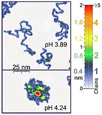


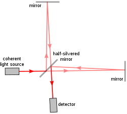


![{\displaystyle (\nu _{2}',\nu _{2})=S^{T}S=\sum _{\nu ^{1}}[S(\nu _{1},\nu _{2}')S(\nu _{1},\nu _{2})],}](https://wikimedia.org/api/rest_v1/media/math/render/svg/27323c6065dc218d72c3453ea490cf30fe8ba063)


